Denoising of Dynamic Contrast-enhanced Ultrasound Sequences: A

Multilinear Approach

Metin Calis

1 a

, Massimo Mischi

2 b

, Alle-Jan Van Der Veen

1 c

and Borb

ala Hunyadi

1 d

Faculty of Electrical Engineering, Mathematics and Computer Science, Delft University of Technology,

2628 CD Delft, The Netherlands

Department of Electrical Engineering, Eindhoven University of Technology, 5600 MB Eindhoven, The Netherlands

Keywords:

Multilinear Singular Value Decomposition, Dynamic Contrast-enhanced Ultrasound, Prostate Cancer, Tensor

Decomposition.

Abstract:

The recent advances in three-dimensional imaging of contrast-enhanced ultrasound acquisitions enable the

characterization of the tissue with a single intravenous injection of microbubbles. Many cancer markers have

been extended to cover for the three-dimensional contrast ultrasound. However, most of the signal denoising

algorithms do not exploit the added dimensionality and vectorize the spatial dimensions, causing a loss of

information about the location of the voxels. This paper proposes a denoising algorithm based on the mul-

tilinear singular value decomposition and compares it to the singular value decomposition. The ranks are

estimated based on information-theoretic criteria, and improved performance has been observed for modeling

the time-intensity curves.

1 INTRODUCTION

Prostate cancer (PCa) is found to be the most com-

mon malignancy among American men except for

skin cancer, and according to the estimates for 2021,

248, 530 new cases are expected of which 34, 130

people will die from the disease (Siegel et al., 2021).

The recommended guidelines for detection and grad-

ing of PCa is ≥ 10-core systematic biopsy (Mottet

et al., 2017), which consists of an invasive procedure

that can still miss signiﬁcant PCa lesions (Ukimura

et al., 2013). In addition, infectious complications

might arise due to the insertion of needles through

the rectal wall (Loeb et al., 2013). Also, because

of the poor patient selection by prostate speciﬁc anti-

gen blood testing, about 3 of 4 biopsies are in retro-

spect unnecessary, as no cancer is found. Recent ad-

vances in imaging techniques can potentially reduce

the needle-cores in systematic biopsy and overcome

unnecessary biopsies (Elwenspoek et al., 2019).

One of the featured techniques to classify PCa

is the detection of angiogenesis, which is the rapid

https://orcid.org/0000-0002-7576-6647

https://orcid.org/0000-0002-1179-5385

https://orcid.org/0000-0003-4249-585X

https://orcid.org/0000-0002-9333-9024

growth of new blood vessels around the tumourous

region. The newly formed capillaries create a tor-

tous and a highly irregular network, that can be an-

alyzed by modelling the ﬂow dynamics of the ul-

trasound contrast agents (UCAs) (Seitz et al., 2009)

(Russo et al., 2012). Although several modalities have

been proposed that can monitor the UCAs, we focus

on dynamic contrast-enhanced ultrasound (DCEUS)

because of the promising results for PCa localization

(Liu et al., 2020) (Wildeboer et al., 2019). In DCEUS,

contrast agents that are smaller than 10 µm are imaged

using a low energy ultrasound pulse. The frequency

of the pulse is around the resonance frequency of

the UCAs, which enhances the contrast between the

microbubbles and the surrounding tissue. The time-

intensity curves (TICs) of these contrast agents corre-

lates with the underlying vasculature (Strouthos et al.,

2010), which can be exploited to classify PCa.

There has been a substantial amount of work in

the analysis of the perfusion characteristics of TICs

(Eckersley et al., 2002) (Elie et al., 2007). Al-

though increased perfusion is expected due to the in-

creased microvascular density, contradictory effects

of angiogenesis and perfusion have been observed

(Gillies et al., 1999). The ﬂow resistance might re-

duce due to the introduction of arteriovenous shunts

and lack of vasomotor control. This effect might

192

Calis, M., Mischi, M., Van Der Veen, A. and Hunyadi, B.

Denoising of Dynamic Contrast-enhanced Ultrasound Sequences: A Multilinear Approach.

DOI: 10.5220/0010838000003123

In Proceedings of the 15th International Joint Conference on Biomedical Engineering Systems and Technologies (BIOSTEC 2022) - Volume 4: BIOSIGNALS, pages 192-199

ISBN: 978-989-758-552-4; ISSN: 2184-4305

not be observed due to the small diameter of the

newly formed microvessels and the increased intersti-

tial pressure because of the extravascular leakage (De-

lorme and Knopp, 1998). A different path has been

taken by (Mischi et al., 2009) (Mischi et al., 2003)

where the authors have modeled the multi-trajectory

bubble transport inside the prostate as a convective-

dispersion process and introduced a new model based

on dispersion characteristics, namely the modiﬁed lo-

cal density random walk model (mLDRW) (Kuenen

et al., 2011). The authors have reported a good cor-

relation between dispersion and angiogenesis even

though the single-dimensional TICs suffer from a low

signal-to-noise (SNR) ratio.

Several techniques were proposed to remove the

noise of various origins from the DCEUS signals.

Spatial ﬁlters were used to denoise the speckle noise

(Bar-Zion et al., 2015) (Joel and Sivakumar, 2018),

temporal ﬁlters were proposed to denoise the clut-

ter (Bjaerum et al., 2002). These methods assumed

that the temporal and spatial frequency of the de-

sired signal and the noise were different. Using a

different approach, the authors at (Wildeboer et al.,

2020) proposed the blind source separation (BSS)

of the DCEUS recording into sources where the de-

sired signal was recovered by discarding the noise

sources. The best performing BSS was found to be

singular value decomposition (SVD) for modelling

of the time intensity curves. The dynamics of the

UCAs have been captured in the ﬁrst few singular val-

ues of the decomposition. Although several cancer

markers such as the similarity between TICs (Schalk

et al., 2015a) and solutions to convective dispersion

models (Wildeboer et al., 2018b) (Wildeboer et al.,

2018a) have been extended to 3D, the denoising algo-

rithms do not take the multidimensional structure of

the recording into consideration.

The SVD denoising analyzed by (Wildeboer et al.,

2020) creates the Casorati matrix, which vectorizes

the spatial dimension into rows and the temporal di-

mension into columns. The vectorization of the spa-

tial dimension into rows results in a loss of spatial

information regarding the location of the voxels. The

multilinear singular value decomposition (MLSVD)

proposed by (De Lathauwer et al., 2000) keeps the

tensor format of the data and generalizes the concept

of SVD to multiple dimensions. The information that

is retained by keeping the tensor format of the data is

hypothesized to enable a better representation of the

bubble dynamics and hence, a better denoising capa-

bility. The MLSVD has been applied for clutter ﬁlter

denoising in power Doppler images (Zhu et al., 2020)

(Ozgun and Byram, 2020). Improved sensitivity and

speciﬁcity have been observed. As far as the authors’

knowledge, there has not been any work done in ana-

lyzing the performance of MLSVD in TIC dispersion

modeling. This paper aims to answer the following

research question: Can the retained 3D structural in-

formation provided by MLSVD improve the classiﬁ-

cation performance of TIC dispersion modeling com-

pared to SVD?

2 BACKGROUND INFORMATION

In this section, the notation is introduced and the mul-

tilinear singular value decomposition (MLSVD) is ex-

plained.

2.1 Notation

The tensor notation of (De Lathauwer et al., 2000) is

adapted in this paper. Tensors are represented with

caligraphic letters, for example, Y and G. The matri-

ces are represented with bold face letters, for example,

(1)

and V. Here, the numbers given as superscripts

in parenthesis are used to refer to the different matri-

ces, that share a similar property. An example could

be the n−mode factor matrices of the same decompo-

sition, which will be explained in the following sub-

section. The scalars are represented with lower case

letters, such as, (A)

i j

= a

i j

and (U)

= u

. The

subscripts refer to the indices in different modalities.

For example, a

i j

refer to the ith row and the jth col-

umn of the matrix A.

2.2 MLSVD

Deﬁnition 1: The casorati matrix is generalized by

the n − mode unfoldings of a tensor. The 1 − mode

unfolding of tensor

Y ∈ R

×N

is represented as Y

(1)

∈

×N

where the columns are the infor-

mation in x direction. Likewise, the 2 − mode

unfolding is Y

(2)

∈ R

×N

, 3 − mode unfolding

is Y

(3)

∈ R

×N

and 4 − mode unfolding is

(4)

∈ R

×N

Deﬁnition 2: The 1-mode product of a matrix U ∈

×N

with Y ∈ R

×N

is a tensor with di-

mension (J

× N

) which has the entries

(Y ×

∑

Likewise, the other n − mode multiplications are de-

ﬁned.

Deﬁnition 3: The scalar product between two tensors

Y , Z ∈ R

×N

hY , Zi =

∑

∗

Denoising of Dynamic Contrast-enhanced Ultrasound Sequences: A Multilinear Approach

193

where

∗

represents the complex conjugate.

Whenever the scalar product between two tensors

is 0, they are orthogonal to each other. The Frobe-

nius norm of a tensor is the square root of the scalar

product of the tensor with itself, ||Y ||

hY , Y i.

Deﬁnition 4: The n-rank of of Y denoted by R

rank

(Y ), is the dimension of the vector space

spanned by the columns of the n − mode unfold-

ing. The multilinear rank for Y is represented as

rank

[]

(Y ) = [R

, R

] where R

, R

are in-

tegers between 1 and N

, N

, respectively.

The MLSVD decomposes the data tensor Y ∈

×N

into

Y = S ×

(1)

(2)

(3)

(4)

where S ∈ R

×N

is an all-orthogonal tensor.

An all-orthogonal tensor has the following properties.

Let a subtensor be deﬁned by ﬁxing an n − mode in-

dex of S. For example let the subtensor created by

ﬁxing the ﬁrst mode value n

∈ [1, ..., N

] to α be

deﬁned as S

=α

. This subtensor S

=α

is orthogo-

nal to any other S

=β

for all n

, α and β given that

α 6= β. In addition, the frobenius norm of each subten-

sor is ordered, ||S

≥ ||S

... ≥ ||S

The matrices U

(1)

∈ R

×N

, U

(2)

∈ R

×N

, U

(3)

∈

×N

and U

(4)

∈ R

×N

are unitary.

3 SIGNAL MODEL

In nearly all commercial scanners the recordings are

logarithmically compressed to deal with the large dy-

namic ranges. Here we model the logarithmically

compressed DCEUS recordings as the addition of the

original signal and the noise,

Y = G + E , (1)

where G ∈ R

×N

stands for the original sig-

nal, Y ∈ R

×N

stands for the received signal

and E ∈ R

×N

stands for the noise. When

only multiplicative noise is considered, and the log-

arithmic compression is applied, E stands for the

speckle noise (Barrois et al., 2013). After the loga-

rithmic compression, speckle noise is shown to obey

the Fisher-Tippet distribution, which can be approx-

imated as a white Gaussian noise with outliers that

has a ﬁxed variance (Michailovich and Tannenbaum,

2006). There can be several other noise sources in

practical scenarios, such as the motion artifacts due

to the urologist’s probe handling and the patient’s

breathing.

The time-intensity curves G are assumed to follow

the modiﬁed local density random walk (mLDRW)

model (Kuenen et al., 2011), which is given as

xyzt

= α

xyz

2π(t −t

)

−

xyz

(t −t

−µ

xyz

)

2(t −t

)

. (2)

Here, κ is the local dispersion-related parameter inde-

pendent of the injection site’s distance. For low values

of dispersion, a symmetric curve and a high κ value

are observed. This is expected to represent malignant

regions (Mischi et al., 2009) (Kuenen et al., 2011).

On the other hand, a low κ is expected to represent

the benign regions.

4 PROPOSED ALGORITHM

The data tensor Y is a 4D DCEUS recording where

the ﬁrst three are the spatial dimensions in the carte-

sian domain, and the fourth is the temporal dimen-

sion. We recover G by truncating Y with ranks

, R

] that obey the condition 1 < R

< N

1 < R

< N

, 1 < R

< N

and 1 < R

< N

. This

assumption is expected to hold since the movement

of the microbubbles is bounded by the spatial loca-

tions of the vascular architecture inside the prostate,

and their temporal characteristics are a latent variable

of indicator dilution models. In addition, we assume

that the noise is independent of the signal itself. With

these assumptions, the problem at hand transforms

into a tensor rank estimation problem, where the rank

that deﬁnes the signal subspace will be estimated, and

the original signal will be recovered.

The multilinear truncation is done on each n −

mode unfolding separately. This can be described as

(1)

= U

(1)

= Σ

(1)

(2)

= U

(2)

= Σ

(2)

(3)

= U

(3)

= Σ

(3)

(4)

= U

(4)

= Σ

(4)

Truncate each singular vector by ﬁrst R

< N

for

i ∈ [x, y, z, t]. This can be described by the operation

(i)

0 Σ

(i)

−R

(i)

(3)

where

(i)

is the column-wise stacking of ﬁrst R

vec-

tors representing the eigenvectors of the highest sin-

gular values,

(i)

is the column-wise stacking of the

− R

columns that represent the eigenvectors of the

rest of the singular values,

(i)

and

(i)

are deﬁned

in a similar way but represent the right eigenvectors

of the ith unfolding of Y .

BIOSIGNALS 2022 - 15th International Conference on Bio-inspired Systems and Signal Processing

194

The multilinear ranks r ank

[]

G are estimated us-

ing the SCORE algorithm proposed by (Yokota et al.,

2016). The truncation is done by projecting each

mode to the column subspace represented by the esti-

mated rank

G = Y ×

(1)

(2)

(3)

(4)

where

G represent the estimate of the TICs.

5 EXPERIMENTAL RESULTS

Two simulations and an in-vivo analysis are reported

in section 5.1 and section 5.2, respectively. In sec-

tion 5.1, a theoretical analysis is done to compare

the performances of SVD and MLSVD for two noise

scenarios. The TICs are generated according to the

model described at (2). The speckle noise is added for

the best-case scenario. Additionally, motion artifacts

and white Gaussian noise are added for the worst-

case scenario. The resulting signals are logarithmi-

cally compressed and then truncated using SVD and

MLSVD. The ranks are estimated using two methods

that are abbreviated as mlsvd min and mlsvd score.

In the former, the rank that gives the least MSE is

chosen and in the latter, the SCORE algorithm pro-

posed by (Yokota et al., 2016) is used. The estimated

signals are ﬁt using the mLDRW model given at (2)

using the algorithm described in (Kuenen et al., 2011)

after reverting the logarithmic compression. For each

algorithm, the mean squared error is calculated by

MSE =

∑

x=1

∑

y=1

∑

z=1

∑

t=1

( ˆg

xyzt

− g

xyzt

)

. (5)

5.1 Simulation

We consider a signal G ∈ R

10×10×10×30

which holds

TICs that obey the mLDRW model as described at

(2). The voxel size is 0.75 mm, and the time step is

4 seconds. The simulated region holds three different

TICs, which have the parameters that are commonly

observed in the literature (Wildeboer et al., 2020), that

is,

• T IC

(κ

, µ

, α

) = [0.5 ±0.1, 30 ± 1, 1000 ± 10] ,

• T IC

(κ

, µ

, α

) = [1 ± 0.1, 25 ± 1, 1600 ± 10] ,

• T IC

(κ

, µ

, α

) = [2 ± 0.1, 15 ± 1, 1200 ± 10] .

Let the ﬁrst malignant region be deﬁned as a

3x3x3 block located at the indices [x, y, z] = [2 : 5, 2 :

5, 2 : 5]. The second malignant region is located at

TIC

1 2 3 4 5 6 7 8 9 10

Figure 1: The simulation setup of 3D rectangular region

with three different TICs. The slice at x = 2 is shown. Three

different simulation areas where the dark blue (majority of

the slice) represents the ﬁrst region, the light blue (left top)

rectangle represents the second region, and the yellow part

(bottom right) represents the third region.

the indices [x, y, z] = [2 : 5, 6 : 9,6 : 9], and the benign

region is the area that is not covered by the ﬁrst two

blocks. A slice at x = 2 represents these three differ-

ent regions, which is given in Figure 1. The benign

region (majority of the block) shown as dark blue is

assigned as region 1, the light blue (left top) rectangle

represents the region 2, and the yellow part (bottom

right) represents the region 3. These numbers are used

for referring to the malignant and benign regions. For

example κ

will refer to the κ values inside the re-

gion 1, κ

for region 2 and κ

for region 3. The other

parameters are represented in the same fashion. The

true rank of the generated signal G in this setup is

rank

[]

G = [2, 3, 3, 3].

Two noise scenarios are simulated. For Scenario

1, the TICs are noised with Rayleigh-shaped multi-

plicative noise. For Scenario 2, a variety of noise

sources have been added. In addition to the multi-

plicative noise, we have added a sinusoidal breath-

ing artifact with an amplitude of 0.5 mm and a fre-

quency of 0.2 Hz, a random-walk displacement that

has the maximum translation of 0.0125 mm at each

step to simulate the probe-handling of the urologist,

white Gaussian noise with 4 dB SNR where the SNR

is calculated with respect to the averaged TICs. For

each case, the error measures given at (5) is calcu-

lated and averaged across 100 Monte Carlo simula-

tions. A plot of MSE can be observed in Figure 2 and

Figure 4 for Scenario 1 and Scenario 2, respectively.

Plot (a) show the MSE over 100 iterations when the

highest 1 to 7 principal components are used for trun-

cation. Since MLSVD does not share the same x axis,

the MSE is drawn as a straight line on the same plot.

The line with the circle markers is the average MSE

over 100 iterations when the best performing trunca-

Denoising of Dynamic Contrast-enhanced Ultrasound Sequences: A Multilinear Approach

195

1 2 3 4 5 6 7

principal components

MSE

(a)

svd

mlsvd_min

mlsvd_score

[2,10,3,3]

[2,3,10,3]

[2,3,3,3]

[2,3,3,6]

[2,3,4,3]

[2,3,5,3]

[2,3,6,3]

[2,3,7,3]

[2,3,9,3]

[2,4,3,3]

[2,4,4,3]

[2,4,5,3]

[2,4,6,3]

[2,4,7,3]

[2,5,3,3]

[2,5,5,3]

[2,6,3,3]

[2,7,3,3]

[2,9,3,3]

counts

(b)

[2,2,2,3]

[2,2,3,3]

[2,3,2,3]

[2,3,3,3]

[2,3,4,3]

[2,4,3,3]

100

counts

(c)

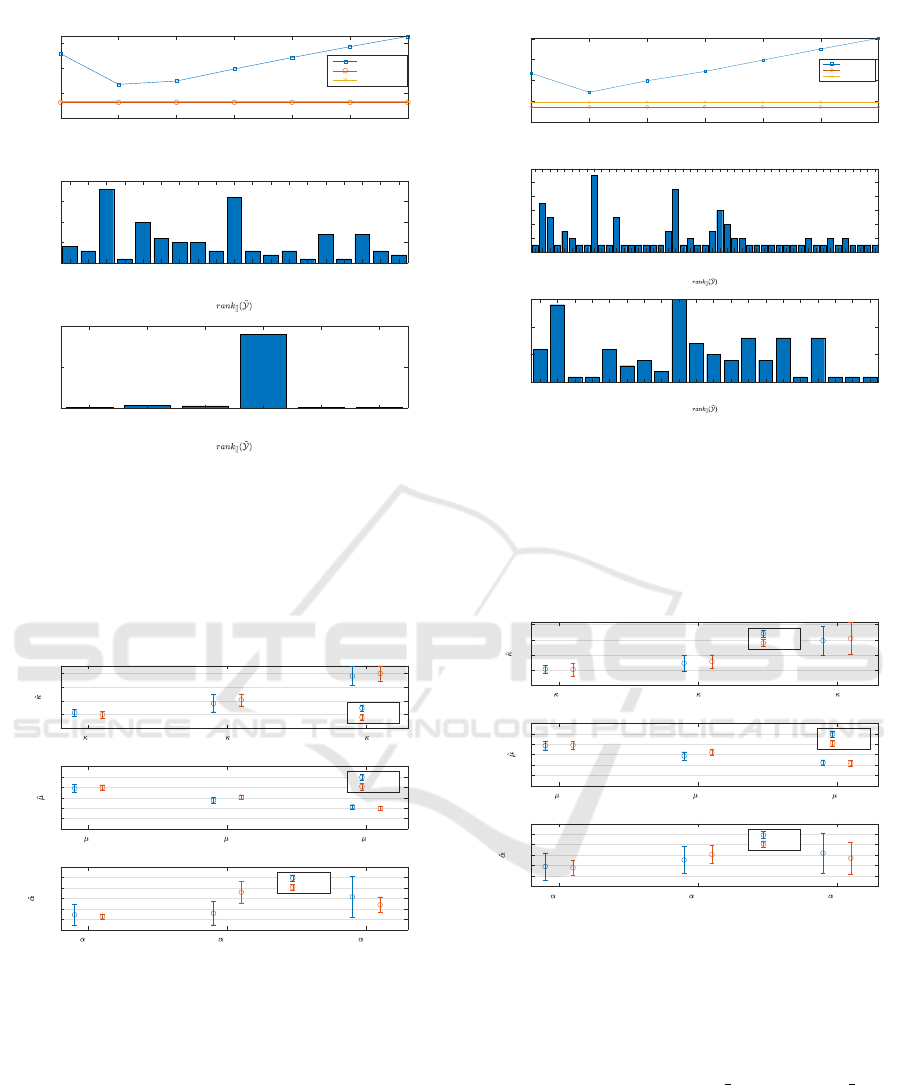
Figure 2: The performance comparison for Scenario 1. At

(a), the MSE of SVD when several principal components

are used to truncate is shown along with two lines that show

the best performing MLSVD error over 100 iterations and

the performance of MLSVD after the ranks are estimated

with SCORE algorithm. At (b), the histogram of the ranks

that gives the least MSE at each simulation is shown. At

(c), the histogram of the ranks that are estimated with the

SCORE algorithm is shown.

TIC

(

= 0.5) TIC

(

= 1) TIC

(

= 2)

TIC curve types

0.5

1.5

svd

mlsvd

TIC

(

= 30) TIC

(

=25) TIC

(

= 15)

TIC curve types

svd

mlsvd

TIC

(

= 1000) TIC

(

= 1600) TIC

(

= 1200)

TIC curve types

800

1000

1200

1400

1600

1800

2000

svd

mlsvd

Figure 3: Plot that shows the mean and the standard devi-

ation of the ˆµ,

κ and

α for three different TICs in Scenario

1. The circles represents the mean values whereas, the error

bars represents the standard deviation. The mean and the

standard deviation are calculated over 100 iterations.

tion is applied, and the line with cross markers is the

MSE when the ranks are estimated using the SCORE

algorithm. Plot (b) and (c) represent the histogram

of the ranks that give the least MSE and the rank esti-

mated by the SCORE algorithm, respectively. The es-

timated κ and µ parameters are shown in Figure 3 and

Figure 5, respectively. In 87 percent of the cases, the

correct rank is estimated by the SCORE algorithm,

1 2 3 4 5 6 7

principal components

100

MSE

(a)

svd

mlsvd_min

mlsvd_score

[2,10,3,3]

[2,3,3,4]

[2,3,4,4]

[2,3,4,5]

[2,3,5,3]

[2,3,5,4]

[2,3,6,3]

[2,3,7,3]

[2,4,3,4]

[2,4,3,5]

[2,4,4,3]

[2,4,4,4]

[2,4,4,5]

[2,4,5,4]

[2,4,6,3]

[2,4,6,4]

[2,4,9,3]

[2,5,2,4]

[2,5,3,3]

[2,5,3,4]

[2,5,3,5]

[2,5,4,4]

[2,5,4,5]

[2,5,5,4]

[2,6,3,3]

[2,6,3,4]

[2,7,3,4]

[2,8,3,3]

[2,8,3,4]

[2,8,5,2]

[2,9,3,3]

[2,9,3,4]

[2,9,4,3]

[3,3,6,2]

[3,5,3,2]

[3,5,4,2]

[3,6,3,2]

[3,7,3,2]

[3,7,3,3]

[3,8,2,2]

[3,8,3,2]

[3,9,3,2]

[4,3,3,2]

[4,4,3,2]

[4,4,4,2]

[7,3,3,2]

[8,3,3,2]

counts

(b)

[3,2,2,3]

[3,2,2,4]

[3,2,2,5]

[3,2,3,3]

[3,2,3,4]

[3,3,2,3]

[3,3,2,4]

[3,3,3,3]

[3,3,3,4]

[4,2,2,3]

[4,2,2,4]

[4,2,3,3]

[4,2,3,4]

[4,3,2,3]

[4,3,2,4]

[4,3,3,3]

[4,3,3,4]

[5,2,2,4]

[5,3,2,4]

[5,3,3,2]

counts

(c)

Figure 4: The performance comparison for Scenario 2. At

(a), the MSE of SVD when several principal components

are used to truncate is shown along with two lines that show

the best performing MLSVD error over 100 iterations and

the performance of MLSVD after the ranks are estimated

with SCORE algorithm. At (b) the histogram of the ranks

that gives the least MSE at each simulation are shown. At

rithm shown.

TIC

(

= 0.5) TIC

(

= 1) TIC

(

= 2)

TIC curve types

0.5

1.5

svd

mlsvd

TIC

(

= 30) TIC

(

= 25) TIC

(

= 15)

TIC curve types

svd

mlsvd

TIC

(

= 1000) TIC

(

= 1600) TIC

(

= 1200)

TIC curve types

800

1000

1200

1400

1600

1800

2000

svd

mlsvd

Figure 5: Plot that shows the mean and the standard devi-

ation of the ˆµ,

κ and

α for three different TICs at Scenario

2. The circles represents the mean values whereas, the error

bars represents the standard deviation. The mean and the

standard deviation are calculated over 100 iterations.

which can be seen at plot (c) of Figure 2. For this

case, the performance of mlsvd min and mlsvd score

overlap suggesting that the SCORE algorithm gives

the least mse over 100 iterations. Although a perfor-

mance improvement over SVD is observed in Figure

4, the ranks are not estimated correctly when a variety

of noise sources are added. The reasons are discussed

at Section 6.

BIOSIGNALS 2022 - 15th International Conference on Bio-inspired Systems and Signal Processing

196

Table 1: The summary of simulation scenarios.

T IC

(κ

, µ

, α

) T IC

(κ

, µ

, α

) T IC

(κ

, µ

, α

)

Number of

Voxels TIC

Number of

Voxels TIC

Number of

Voxels TIC

Noise Types

Number of

Simulations

Scenario 1 (0.5 ± 0.1,30 ± 1, 1000 ± 10) (1 ± 0.1, 25 ± 1, 1600 ± 10) (2 ± 0.1, 15 ± 1, 1200 ± 10) 872 64 64 Multiplicative 100

Scenario 2 (0.5 ± 0.1,30 ± 1, 1000 ± 10) (1 ± 0.1, 25 ± 1, 1600 ± 10) (2 ± 0.1, 15 ± 1, 1200 ± 10) 872 64 64

Multiplicative,

Breathing, Motion,

WGN

100

Table 2: The estimated model ﬁt parameters across all pa-

tients.

SVD

MLSVD-SCORE

ρ = 10e − 4

Benign Malignant Benign Malignant

κ 0.51(σ = 0.35) 0.56(σ = 0.33) 0.39(σ = 0.18) 0.48(σ = 0.22)

PV 94.73(σ = 29.57) 104.05(σ = 27.53) 87.87(σ = 26.33) 98.49(σ = 24.03)

PT 33.76(σ = 9.57) 30.00(σ = 8.09) 32.56(σ = 6.95) 29.24(σ = 5.62)

AT 15.12(σ = 4.96) 13.72(σ = 4.23) 14.32(σ = 3.44) 13.41(σ = 3.11)

WIT 18.64(σ = 9.41) 16.28(σ = 7.44) 18.24(σ = 5.91) 15.84(σ = 4.08)

µ 35.28(σ = 11.48) 31.31(σ = 9.57) 34.29(σ = 8.31) 30.58(σ = 6.24)

α 172.99(σ = 126.38) 184.39(σ = 123.05) 143.78, (σ = 77.96) 154.09, (σ = 68.92)

Table 3: The classiﬁcation performance across all the pa-

tients.

SVD

MLSVD-SCORE

(ρ = 10e − 4)

[κ

sens

, κ

spec

, κ

AUC

,threshold] [0.54,0.53,0.57,0.51] [0.48,0.65,0.63,0.45]

[PI

sens

, PI

spec

, PI

AUC

,threshold] [0.60,0.54,0.61,99] [0.63,0.57,0.64,93]

[PT

sens

, PT

spec

, PT

AUC

,threshold] [0.57,0.62,0.61,31] [0.59,0.65,0.63,30]

[α

sens

, α

spec

, α

AUC

,threshold] [0.54,0.51,0.55,150] [0.46,0.64,0.58,160]

[W IR

sens

,W IR

spec

,W IR

AUC

,threshold] [0.58,0.59,0.63,6.6] [0.62,0.59,0.66,5.7]

[AT

sens

, AT

spec

, AT

AUC

,threshold] [0.65,0.58,0.59,15] [0.72,0.59,0.58,13.8]

[W IT

sens

,W IT

spec

,W IT

AUC

,threshold] [0.58,0.57,0.56,16] [0.59,0.58,0.62,16.5]

5.2 In-vivo Analysis

The recording of 6 patients was acquired from the

Second Afﬁliated Hospital of Zheijang University

(Hangzhou, Zheijang, China). Written consent was

obtained. A 2.4-mL bolus of SonoVue

was in-

travenously injected, and a 4D recording in con-

trast mode was obtained with a LOGIQ E9 scanner

equipped with a RIC5-9-D endocavitary transducer

driven at 4 MHz. The volume rate was ﬁxed to 0.25

Hz by setting the image quality to low, and the dis-

ruption of microbubbles was avoided by ﬁxing the

mechanical index to 0.1. The patients went through

prostatectomy after the recording. The prostate was

sliced with 4-mm thickness, and for each slice, an

annotation was made by the pathologist. The an-

notations were registered back to the domain of the

recording, and the ground truth was obtained. Only

two out of the six patients had signiﬁcant lesions with

Grade Group > 3. A region of interest is selected in

the benign and malignant regions that are reasonably

close to the true annotations. There are around 25000

voxels, of which 18000 are malignant.

The spatial resolution of the recording is regular-

ized in space, and the data is downsampled by a fac-

tor of 3 as described by (Schalk et al., 2015b). The

MLSVD is applied, and the signal is truncated us-

ing the ranks estimated by the SCORE (Yokota et al.,

2016) algorithm where ρ = 10e − 4 is selected. The

mLDRW model is ﬁt as described at (Kuenen et al.,

2011), and the perfusion and dispersion parameters

are extracted. The results can be seen in Table 2 and

Table 3. In the former, the mean and the standard de-

viation of the features are shown. In the latter, the

sensitivity, speciﬁcity, and area under the receiver op-

erating characteristic curves are shown. The classiﬁ-

cation is done by determining the point in the receiver

operating characteristic curve that is the closest to the

upper left corner (sensitivity and speciﬁcity equal to

1) in Euclidean distance.

6 DISCUSSION

In this paper, the DCEUS sequences are denoised us-

ing SVD and MLSVD, and their performances are

evaluated based on the quality of the TIC model-

ing. In section 5.1, two simulations are reported that

employ the commonly observed noises in DCEUS

recordings. The ﬁrst simulation represents the best-

case scenario where only speckle-noise exists. The

second simulation represents the worst-case scenario

where additive WGN and motion exist apart from

the speckle noise. MLSVD mostly performs better

at capturing the signal characteristics in both cases,

providing a better estimate of dispersion and perfu-

sion parameters. Both methods perform worse in the

worst-case scenario and fail to estimate high κ values

precisely. The low SNR might explain the decrease in

performance.

The speckle noise can be modeled as a WGN

with outliers (Michailovich and Tannenbaum, 2006),

which results in the correct estimation of the rank for

Scenario 1. The actual rank of the signal is [2, 3, 3, 3],

which is the same as the rank that is estimated the

majority of the time. For this case, we can see in Fig-

ure 2 that the MSE of the best performing rank and

the estimated rank overlap. In the cases where the

rank was incorrectly estimated, the error is found to

be within 15% of the MSE represented with the line

mlsvd score. The estimation of the correct rank fails

for Scenario 2. Adding the other noise sources vio-

lates the WGN assumption and causes the rank esti-

mator to perform poorly. This suggests that in a prac-

tical scenario where the recording suffers from var-

ious noise sources apart from the speckle noise, the

proposed algorithm might not be suitable. In the ﬁg-

ures Figure 2 and Figure 4, it can be observed that the

best performing rank is not necessarily the true rank

Denoising of Dynamic Contrast-enhanced Ultrasound Sequences: A Multilinear Approach

197

of the data. The subﬁgures labeled with (b) in both

plots suggest that the noise in some cases might oc-

cupy the highest ranks. For this reason, a higher rank

might have provided a lower MSE.

Better classiﬁcation performance of MLSVD over

SVD is observed at Table 3. The improvement is more

signiﬁcant when a subset of the patients is considered.

This might be due to the insigniﬁcant malignant vox-

els of the four patients that are investigated. The sig-

niﬁcant malignant lesions are expected to have a more

distinct characteristic than benign tissue. This behav-

ior is observed for two of the patients, who have sig-

niﬁcant lesions. The AUC is found to be greater than

0.8 for these two patients whereas, a similar perfor-

mance has not been observed for the others.

7 CONCLUSION

In this paper, we proposed a denoising algorithm for

detecting prostate cancer from 4D DCEUS record-

ings. Previously, SVD was proposed to denoise the

single-dimensional TICs that suffer from low SNR.

Here, we have retained the volumetric information

by considering the tensor format of the recording

and introduced an algorithm based on MLSVD and

SCORE. The proposed algorithm is shown to outper-

form SVD in simulation and in in-vivo experiments.

The in-vivo results have poor classiﬁcation perfor-

mance, which can be due to the insigniﬁcant lesions

found in four of the six patients that have undergone

prostatectomy. In future work, we plan to use a larger

dataset and include other features used in the detec-

tion of angiogenesis.

ACKNOWLEDGEMENTS

This project is funded in part by Holland High Tech

with a PPS supplement for research and development

in the Topsector HTSM. We would like to acknowl-

edge Prof. Pintong Huang for carrying out the clini-

cal trials at the Second Afﬁliated Hospital of Zheijang

University (Hangzhou, Zheijang, China).

REFERENCES

Bar-Zion, A. D., Tremblay-Darveau, C., Yin, M., Adam,

D., and Foster, F. S. (2015). Denoising of contrast-

enhanced ultrasound cine sequences based on a mul-

tiplicative model. IEEE Transactions on Biomedical

Engineering, 62(8):1969–1980.

Barrois, G., Coron, A., Payen, T., Dizeux, A., and Bridal,

L. (2013). A multiplicative model for improving

microvascular ﬂow estimation in dynamic contrast-

enhanced ultrasound (dce-us): theory and experimen-

tal validation. IEEE transactions on ultrasonics, fer-

roelectrics, and frequency control, 60(11):2284–2294.

Bjaerum, S., Torp, H., and Kristoffersen, K. (2002). Clutter

ﬁlter design for ultrasound color ﬂow imaging. IEEE

Transactions on Ultrasonics, Ferroelectrics, and Fre-

quency Control, 49(2):204–216.

De Lathauwer, L., De Moor, B., and Vandewalle, J.

(2000). A multilinear singular value decomposition.

SIAM journal on Matrix Analysis and Applications,

21(4):1253–1278.

Delorme, S. and Knopp, M. (1998). Non-invasive vascu-

lar imaging: assessing tumour vascularity. European

radiology, 8(4):517–527.

Eckersley, R. J., Sedelaar, J. M., Blomley, M. J., Wijk-

stra, H., deSouza, N. M., Cosgrove, D. O., and de la

Rosette, J. J. (2002). Quantitative microbubble en-

hanced transrectal ultrasound as a tool for monitor-

ing hormonal treatment of prostate carcinoma. The

Prostate, 51(4):256–267.

Elie, N., Kaliski, A., P

eronneau, P., Opolon, P., Roche, A.,

and Lassau, N. (2007). Methodology for quantify-

ing interactions between perfusion evaluated by dce-

us and hypoxia throughout tumor growth. Ultrasound

in medicine & biology, 33(4):549–560.

Elwenspoek, M. M. C., Sheppard, A. L., McInnes, M. D. F.,

Merriel, S. W. D., Rowe, E. W. J., Bryant, R. J.,

Donovan, J. L., and Whiting, P. (2019). Compari-

son of Multiparametric Magnetic Resonance Imaging

and Targeted Biopsy With Systematic Biopsy Alone

for the Diagnosis of Prostate Cancer: A Systematic

Review and Meta-analysis. JAMA Network Open,

2(8):e198427–e198427.

Gillies, R. J., Schomack, P. A., Secomb, T. W., and Raghu-

nand, N. (1999). Causes and effects of heterogeneous

perfusion in tumors. Neoplasia, 1(3):197–207.

Joel, T. and Sivakumar, R. (2018). An extensive review

on despeckling of medical ultrasound images using

various transformation techniques. Applied Acoustics,

138:18–27.

Kuenen, M. P. J., Mischi, M., and Wijkstra, H. (2011).

Contrast-ultrasound diffusion imaging for localization

of prostate cancer. IEEE Transactions on Medical

Imaging, 30(8):1493–1502.

Liu, G., Wu, S., and Huang, L. (2020). Contrast-enhanced

ultrasound evaluation of the prostate before transrectal

ultrasound-guided biopsy can improve diagnostic sen-

sitivity: A stard-compliant article. Medicine, 99(19).

Loeb, S., Vellekoop, A., Ahmed, H. U., Catto, J., Ember-

ton, M., Nam, R., Rosario, D. J., Scattoni, V., and

Lotan, Y. (2013). Systematic review of complications

of prostate biopsy. European Urology, 64(6):876–892.

Michailovich, O. and Tannenbaum, A. (2006). Despeckling

of medical ultrasound images. IEEE Transactions on

Ultrasonics, Ferroelectrics, and Frequency Control,

53(1):64–78.

BIOSIGNALS 2022 - 15th International Conference on Bio-inspired Systems and Signal Processing

198

Mischi, M., Kalker, A., and Korsten, H. (2003). Video-

densitometric methods for cardiac output measure-

ments. EURASIP Journal on Applied Signal Process-

ing, 2003(5):479–489.

Mischi, M., Kuenen, M., Wijkstra, H., Hendrikx, A., and

Korsten, H. (2009). Prostate cancer localization by

contrast-ultrasound diffusion imaging. In 2009 IEEE

International Ultrasonics Symposium, pages 283–

286.

Mottet, N., Bellmunt, J., Bolla, M., Briers, E., Cumber-

batch, M. G., De Santis, M., Fossati, N., Gross, T.,

Henry, A. M., Joniau, S., Lam, T. B., Mason, M. D.,

Matveev, V. B., Moldovan, P. C., van den Bergh, R. C.,

Van den Broeck, T., van der Poel, H. G., van der

Kwast, T. H., Rouvi

ere, O., Schoots, I. G., Wiegel, T.,

and Cornford, P. (2017). Eau-estro-siog guidelines on

prostate cancer. part 1: Screening, diagnosis, and lo-

cal treatment with curative intent. European Urology,

71(4):618–629.

Ozgun, K. and Byram, B. (2020). A channel domain higher-

order svd clutter rejection ﬁlter for small vessel ultra-

sound imaging. In 2020 IEEE International Ultrason-

ics Symposium (IUS), pages 1–4.

Russo, G., Mischi, M., Scheepens, W., De la Rosette, J. J.,

and Wijkstra, H. (2012). Angiogenesis in prostate can-

cer: onset, progression and imaging. BJU Interna-

tional, 110(11c):E794–E808.

Schalk, S. G., Demi, L., Smeenge, M., Mills, D. M., Wal-

lace, K. D., de la Rosette, J. J. M. C. H., Wijkstra, H.,

and Mischi, M. (2015a). 4-d spatiotemporal analy-

sis of ultrasound contrast agent dispersion for prostate

cancer localization: a feasibility study. IEEE Trans-

actions on Ultrasonics, Ferroelectrics, and Frequency

Control, 62(5):839–851.

Schalk, S. G., Demi, L., Smeenge, M., Mills, D. M., Wal-

lace, K. D., de la Rosette, J. J. M. C. H., Wijkstra, H.,

and Mischi, M. (2015b). 4-d spatiotemporal analy-

sis of ultrasound contrast agent dispersion for prostate

cancer localization: a feasibility study. IEEE Trans-

actions on Ultrasonics, Ferroelectrics, and Frequency

Control, 62(5):839–851.

Seitz, M., Shukla-Dave, A., Bjartell, A., Touijer, K., Scia-

rra, A., Bastian, P. J., Stief, C., Hricak, H., and Graser,

A. (2009). Functional magnetic resonance imaging in

prostate cancer. European Urology, 55(4):801–814.

Siegel, R. L., Miller, K. D., Fuchs, H. E., and Jemal, A.

(2021). Cancer statistics, 2021. CA: A Cancer Journal

for Clinicians, 71(1):7–33.

Strouthos, C., Lampaskis, M., Sboros, V., McNeilly, A., and

Averkiou, M. (2010). Indicator dilution models for the

quantiﬁcation of microvascular blood ﬂow with bolus

administration of ultrasound contrast agents. IEEE

transactions on ultrasonics, ferroelectrics, and fre-

quency control, 57(6):1296–1310.

Ukimura, O., Coleman, J. A., de la Taille, A., Emberton,

M., Epstein, J. I., Freedland, S. J., Giannarini, G., Ki-

bel, A. S., Montironi, R., Ploussard, G., Roobol, M. J.,

Scattoni, V., and Jones, J. S. (2013). Contemporary

role of systematic prostate biopsies: Indications, tech-

niques, and implications for patient care. European

Urology, 63(2):214–230.

Wildeboer, R., Van Sloun, R., Mannaerts, C., Van der Lin-

den, J., Huang, P., Wijkstral, H., and Mischi, M.

(2018a). Probabilistic 3d contrast-ultrasound trac-

tography based on a a convective-dispersion ﬁnite-

element scheme. In 2018 IEEE International Ultra-

sonics Symposium (IUS), pages 1–9.

Wildeboer, R. R., Sammali, F., van Sloun, R. J. G., Huang,

Y., Chen, P., Bruce, M., Rabotti, C., Shulepov, S., Sa-

lomon, G., Schoot, B. C., Wijkstra, H., and Mischi, M.

(2020). Blind source separation for clutter and noise

suppression in ultrasound imaging: Review for differ-

ent applications. IEEE Transactions on Ultrasonics,

Ferroelectrics, and Frequency Control, 67(8):1497–

1512.

Wildeboer, R. R., van Sloun, R. J., Huang, P., Wijkstra,

H., and Mischi, M. (2019). 3-d multi-parametric

contrast-enhanced ultrasound for the prediction of

prostate cancer. Ultrasound in medicine & biology,

45(10):2713–2724.

Wildeboer, R. R., Van Sloun, R. J. G., Schalk, S. G.,

Mannaerts, C. K., Van Der Linden, J. C., Huang, P.,

Wijkstra, H., and Mischi, M. (2018b). Convective-

dispersion modeling in 3d contrast-ultrasound imag-

ing for the localization of prostate cancer. IEEE Trans-

actions on Medical Imaging, 37(12):2593–2602.

Yokota, T., Lee, N., and Cichocki, A. (2016). Robust multi-

linear tensor rank estimation using higher order sin-

gular value decomposition and information criteria.

IEEE Transactions on Signal Processing, 65(5):1196–

1206.

Zhu, Y., Kim, M., Hoerig, C., and Insana, M. F. (2020). Ex-

perimental validation of perfusion imaging with hosvd

clutter ﬁlters. IEEE Transactions on Ultrasonics, Fer-

roelectrics, and Frequency Control, 67(9):1830–1838.

Denoising of Dynamic Contrast-enhanced Ultrasound Sequences: A Multilinear Approach

199