
Non-planar Surface Shape Reconstruction from a Point Cloud in the
Context of Muscles Attachments Estimation
∗
Josef Kohout
a
and Martin Cervenka
b
Faculty of Applied Sciences, University of West Bohemia, Technick
´
a 8, Plze
ˇ
n, Czech Republic
Keywords:
Shape Reconstruction, Point Cloud, Multidimensional Scaling, Muscle Attachments Estimation, Fast March-
ing, Scalar Distance Field.
Abstract:
Knowledge of muscle attachments on bones is essential for musculoskeletal modelling. A muscle attachment
is often represented by points (in 3D) obtained by a manual digitisation system during dissection. Although
this representation suffices for many purposes, sophisticated musculoskeletal models commonly require repre-
senting a muscle attachment by a surface patch or at least by a closed boundary curve. In this paper, therefore,
we propose an approach to automatic shape reconstruction from such point sets. It is based on iso-contour
extraction from a scalar field of distances to geodetics connecting the pairs of points (from the input set) as
identified by a state-of-the-art algorithm for 2D curve reconstruction running on the input points transformed
to 2D. We investigated the performance of 15 existing state-of-the-art algorithms with public implementations
on the TLEM 2.0 data set of muscle attachments. The best results were obtained for the lenz algorithm with
just one unacceptable reconstruction when standard projection onto a best-fit plane was used to transform the
input 3D points to 2D. The second algorithm was α-shape with three unacceptable reconstructions, whereas
in this case, the multidimensional scaling technique was exploited to transform the points.
1 INTRODUCTION
Shape reconstruction from a point cloud is an im-
portant computational geometry problem with vari-
ous applications in computer graphics, computer vi-
sion, medical image analysis, pattern recognition,
computer-aided design, cultural heritage, and others.
During the past decades of research, many algorithms
for shape reconstruction have been proposed. Some
work with points sampled on the boundary of an ob-
ject whose shape is to reconstruct, while others work
with the points sampled in its interior . Some algo-
rithms can deal (to some extent) with non-uniform or
sparse sampling, noise or outliers , while others as-
sume a dense uniform sampling Some focus on spe-
cific kinds of objects, e.g., CAD objects with sharp
edges or terrain data . Some require additional infor-
mation, such as normals in points . However, most
importantly, some work in 2D, processing 2D point
a
https://orcid.org/0000-0002-3231-2573
b
https://orcid.org/0000-0001-9625-1872
∗
This Work Was Supported by the Meys of the Czech
Republic, Project SGS-2019-016.
†
Corresponding author
clouds to reconstruct the outlining contour of the ob-
ject, while others work in 3D, processing 3D point
clouds to reconstruct the outlining surface of the ob-
ject. A good survey of algorithms of the former cate-
gory can be found in (Ohrhallinger et al., 2021). For
a survey of the algorithms of the latter category, we
refer the reader to (Berger et al., 2016).
In this paper, we propose a novel algorithm for re-
constructing a space curve from a set of 3D points. It
employs the multidimensional scaling technique (Cox
and Cox, 2008) to transform the points from 3D to 2D
and then uses a suitable algorithm for 2D curve recon-
struction to get the connectivity of the input points.
Motivation for our work lies in muscle attach-
ment estimation. Knowledge of muscle attachments
on bones is essential for musculoskeletal modelling.
A muscle attachment is often represented by points
obtained by a manual digitisation system during dis-
section. Due to the apparent effort associated with
this process, no wonder that the sampling is sparse.
Commonly, the points are unordered and exhibit a
non-uniform distribution because it is natural to sam-
ple the upper side of the attachment area from left to
right, then cut off the muscle-tendon unit and sample
the lower side from left to right. The points are sub-
236
Kohout, J. and Cervenka, M.
Non-planar Surface Shape Reconstruction from a Point Cloud in the Context of Muscles Attachments Estimation.
DOI: 10.5220/0010869600003124
In Proceedings of the 17th International Joint Conference on Computer Vision, Imaging and Computer Graphics Theory and Applications (VISIGRAPP 2022) - Volume 1: GRAPP, pages
236-243
ISBN: 978-989-758-555-5; ISSN: 2184-4321
Copyright
c
2022 by SCITEPRESS – Science and Technology Publications, Lda. All rights reserved

ject to various errors, introduced during the dissection
(e.g., movements of the limbs, the ambiguity in defin-
ing the attachment boundary) or during the registra-
tion process. Sometimes a few points are even sam-
pled in the interior of the attachment area. Figure 1
shows an example of such data.
Figure 1: TLEM 2.0 (Carbone et al., 2015) data set con-
taining point clouds defining various muscle attachments on
lower limbs.
It can be seen that the attachment areas are only
slightly curved. Therefore, a naive approach would
be to project the points onto the best-fitted plane (ob-
tained, e.g., by using the least-squares method) and
then proceed with some of the existing state-of-the-art
algorithms for reconstructing 2D curves. This paper
investigates if exploiting the multidimensional scal-
ing (MDS) technique would not improve the obtained
results when comparing them with the ground truth.
We experimented with 15 different algorithms.
Our other contribution is as follows. Since the
3D models of bones are available, we propose an ap-
proach to convert a non-manifold curve, which may
result from the process, into a closed manifold one. It
is based on iso-contour extraction from the scalar field
on the surface of the bones that encodes distances to
geodetics connecting the adjacent points of curves.
2 RELATED WORK
The problem of muscle attachments estimation was
addressed in (Fukuda et al., 2017). The authors dis-
sected individual muscles in the hip region of eight
cadaver specimens while tracing the boundary of the
muscle attachments using an optical tracker. The
recorded points were manually refined to remove out-
lier measurements due to tracking noise. In this paper,
we investigate if we could get the boundary of an at-
tachment automatically without the necessity of such
manual refinement.
In their work, (Kohout and Kuka
ˇ
cka, 2014) de-
scribed a fully automatic algorithm for extraction of
a closed region from a triangular model of a muscle,
where region boundary is specified by a set of points
lying on the muscle surface or in its vicinity. The
points had to be specified in an order such that inter-
connecting every pair of adjacent points by a line seg-
ment would produce a closed non-intersecting poly-
line corresponding to the boundary of the region to
extract. However, typical data sets of attachment ar-
eas do not comply with this requirement, as shown
in Figure 1. In this paper, we investigate how to fil-
ter out the input points and order them to satisfy the
requirement of this algorithm.
Approximating or interpolating the input points by
an analytical function may be considered relevant to
this problem. Most suitable seems to be radial ba-
sis function (RBF) approximation since the points are
scattered and unordered. RBF was used for surface
reconstruction of watertight 3D objects by (Carr et al.,
2001). It is also commonly used for scattered data ap-
proximation in general (Cervenka et al., 2019). In this
paper, we address the idea of transforming the input
3D points to 2D, finding the curve there (by exploit-
ing RBF approximation) and returning to 3D space.
One option for the points dimension reduction is the
multidimensional scaling (MDS) technique (Cox and
Cox, 2008), which is widely used in many different
scientific fields.
Recently, (Ohrhallinger et al., 2021) designed a
benchmark for a comprehensive quantitative evalua-
tion of algorithms for 2D curves reconstruction. It
consists of 14 curve reconstruction algorithms, in-
cluding the recent ones, implemented in C++. Most
of these algorithms construct a graph from the points
and then filter the outline by some criteria. Most of
them are parameterless, but only some are robust to
noise and outliers.
3 OUR APPROACH
Given a set S = (P
i
) of n points in 3D, sampled on
a smooth curve on a non-planar smooth surface, in-
cluding potentially noise or outliers, our task is to find
an ordered set S
0
⊆ S such that S
0
represents a closed
non-intersecting space curve. The other points (S \S
0
)
which do not lie on the curve are considered as out-
liers. Figure 2 shows an example of the input data.
Our basic idea is to exploit the multidimensional
scaling (MDS) technique (Cox and Cox, 2008) to con-
struct n points Q
i
in 2D such that:
Non-planar Surface Shape Reconstruction from a Point Cloud in the Context of Muscles Attachments Estimation
237

Figure 2: Obturator internus origin data set. Left - the input
point set together with the order in which the points were
sampled, right - the ground truth closed curve we specified
manually according to anatomical atlases.
• every point Q
i
is uniquely associated with just one
point P
i
so we are able to return back to 3D, and
• the distance between a pair of points Q
i
, Q
j
are as
close to the distance between a pair of associated
points P
i
, P
j
as possible.
Executing a 2D curve reconstruction algorithm on
the set of points Q
i
produces the sought connectivity
between the points P
i
. If the output connectivity forms
a single closed curve, we are ready. Otherwise, the
output must be filtered: some edges might need to be
removed, some edges to close the curve might need to
be inserted. We assume that the surface from which
the data were sampled is available and is represented
by a triangular model, or can be reconstructed from
the input points, e.g., by using the RBF approach (see
Section 3.1). It allows us to solve the filtering step in
a rather unorthodox but straightforward approach.
Suppose the points P
i
and P
j
should be connected.
At first, we subdivide the triangles of the surface mesh
that contain these points in their vicinity, introduc-
ing thus these points as new vertices of the mesh.
Then, we trace the shortest path connecting newly in-
troduced vertices to a set of surface points P
i, j,k
, as
illustrated in Figure 3. The Dijkstra algorithm can be
used for it, providing that the triangular model is fine
enough. Some of the fast marching methods, see, e.g.,
(Peyr
´
e, 2009), is an alternative suitable in all cases.
We construct a scalar field SDF(V ) on the surface
of the mesh such that it returns the geodetic distance
between the given surface point V and the nearest
P
i, j,k
point – see Figure 4. This field can be con-
structed easily using a bread-first search algorithm
starting at P
i, j,k
points. We adopt a fast marching
method described in (Peyr
´
e, 2009) for this purpose.
An algorithm for iso-contours extraction is ex-
ecuted with the iso-value about the average length
of edges P
i, j,k
, P
i, j,k+1
. In our experiments, we
specify this value to 0.5 · (minkP
i, j,k
, P
i, j,k+1
k +
maxkP
i, j,k
, P
i, j,k+1
k). Multiple contours are usually
P
18,19,0
P
18,19,1
P
18,19,2
P
18,19,3
P
18,19,4
P
18,19,5
P
18,19,0
P
27,18,0
P
27,18,6
P
27,18,6
P
27,18,7
P
27,18,8
P
17,27,0
P
17,27,0
P
17,27,1
P
17,27,2
P
17,27,3
P
17,27,4
P
17,27,5
P
17,27,6
P
17,27,7
Figure 3: Refined edges P
17
, P
27
, P
27
, P
18
, and P
18
, P
19
of
the obturator internus origin data set (see Figure 2) on the
surface of the pelvis bone.
Figure 4: Scalar field constructed on the surface of the
pelvis bone for the refined connectivity (obtained by (Lenz,
2006) algorithm) of the obturator internus origin data set.
extracted (e.g., one from the exterior of a closed
curve, the other from the interior). The one with the
largest perimeter is selected as a result – see Figure 5
for an example. We note that the final contour does
not go through the input points but providing that the
refinement of the primary edges is sufficient, this does
not stand for a problem in many applications (includ-
ing the muscle attachments estimation).
3.1 Radial Basis Functions (RBF)
Radial basis function interpolation and approximation
is defined as follows:
h
i
(x) =
N
∑
j=1
λ
j
ϕ(|||x
i
− x
j
||), (1)
or also: h = Aλ, A
i, j
= ϕ(||x
i
− x
j
||)
The λ
i
variable is the weight of a single RBF, ϕ de-
notes radial basis function, x
i
and x
j
are the positions
of the input vertices (maybe attachment area vertices
in our case), and h
i
are values in the vertices.
GRAPP 2022 - 17th International Conference on Computer Graphics Theory and Applications
238
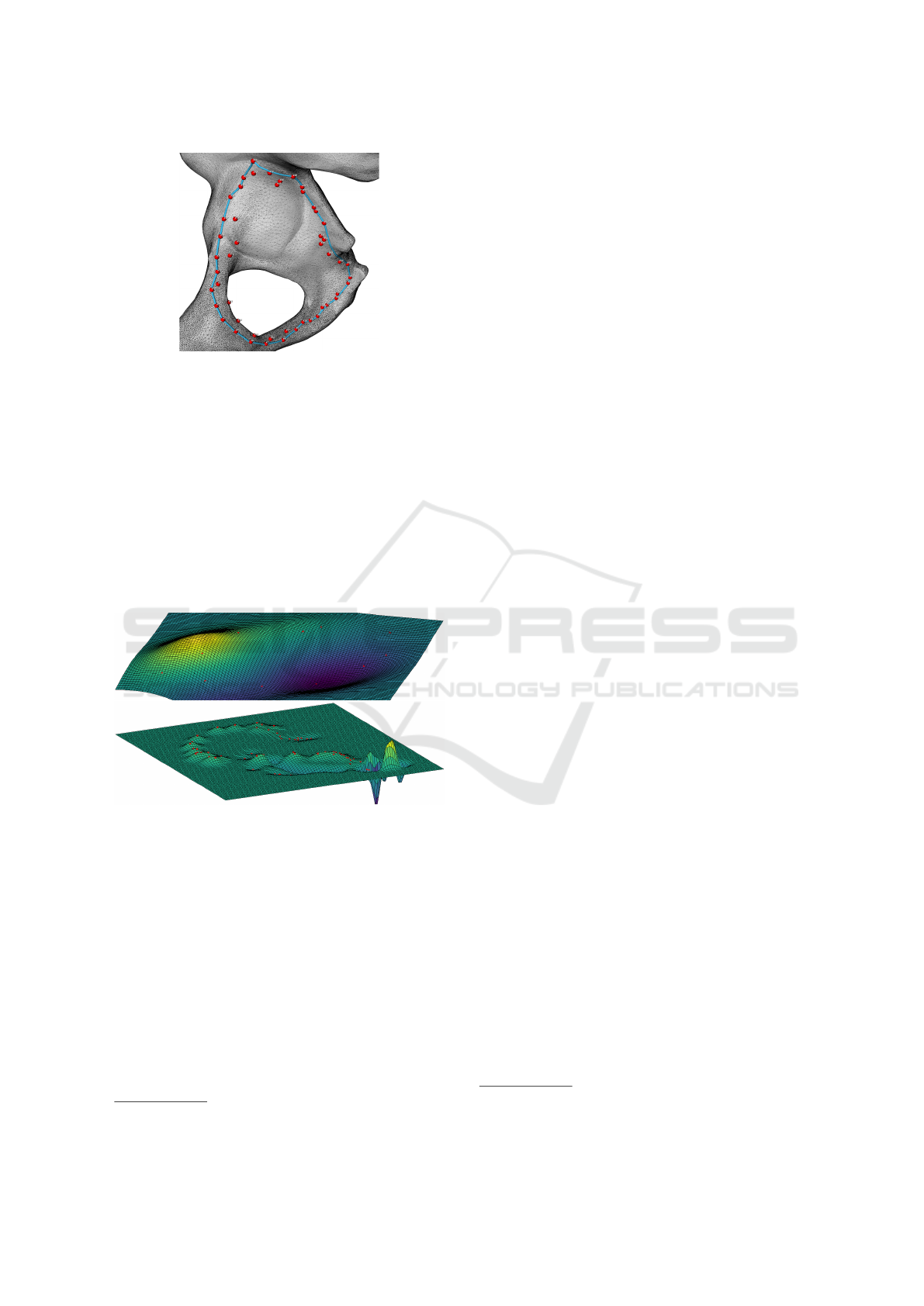
Figure 5: Obturator internus origin closed curve extracted
from the scalar field in Figure 4. Compare it with the ground
truth curve in Figure 2 right.
We experimented with a novel RBF described in
(Skala and Cervenka, 2020) defined as:
ϕ(r) = r
2
(r
a
− 1) (2)
Variable a is a shape parameter that has to be iden-
tified accurately to get good results. We also used
a = 1.8 as proposed by the original authors. Fig-
ure 6 shows the surface reconstructed by this ap-
proach from the input points. This surface can be used
as an alternative to the triangulated model of a bone.
Figure 6: The surface of the femur bone reconstructed by
the RBF method from the input points of biceps femoris
origin (top) and vastus intermedius origin (bottom).
4 EXPERIMENTS AND RESULTS
The approach described above was implemented in
C++ 14 using:
• the Visualization Toolkit (VTK)
1
for loading the
data, curve reconstruction by the α-shape algo-
rithm (see (Edelsbrunner et al., 1983)), iso-lines
extraction , and visualization of results,
• the benchmarking by (Ohrhallinger et al., 2021)
for curve reconstruction by 14 different algo-
1
https://vtk.org/
rithms – connect2d, hnncrust, fitconnect, stretch-
denoise, discur, vicur, crawl, peel, crust, nncrust,
ccrust, gathan1, gathang, and lenz,
• the code by Yuki Koyama
2
for the multidimen-
sional scaling,
• the geodesic computation on surfaces by (Krish-
nan, 2013), based on the fast marching method,
• and the Muscle Decomposition by (Kohout and
Kuka
ˇ
cka, 2014) for extracting the muscle attach-
ment area bounded by the reconstructed curve
from the surface mesh.
We note that the disk radius parameter of the α-shape
algorithm was set to 0.5625 times the maximal short-
est distance between pairs of points, i.e., just enough
to guarantee that the output will have one component
only. The implementations of the other reconstruction
algorithms were used with their default parameters.
We experimented with the point sets representing
muscle attachments of a comprehensive TLEM 2.0
data set of lower limbs (Carbone et al., 2015). Af-
ter performing initial analyses, we selected, more or
less randomly, a couple of representative point sets for
further experiments – see Figure 7. For each of the 27
point sets we ended with, we specified the ground-
truth connection of the points according to depictions
in anatomical atlases. We note that in some cases, the
task of finding a proper connection has proven to be
complicated even for a human expert.
We inserted the points into the surface mesh of the
appropriate bone and used the geodesic computation
to obtain the final closed ground-truth curve. An ex-
ample of such a curve is in Figure 2, right.
Using the code for the muscle decomposition by
(Kohout and Kuka
ˇ
cka, 2014), we extracted the part of
the mesh belonging to the attachment area bounded
by the ground-truth closed curve. In three cases (ad-
ductor longus insertion, obturator internus origin and
gluteus maximus inferior origin), the implementation
failed to provide us with an acceptable result. This
was caused by the fact that the input data violated the
assumptions of the original method. Figure 8 shows
examples of extracted ground-truth attachments.
We then ran our implementation. It provided us
with 15 contours for each dataset, one for every curve
reconstruction algorithm. For each output contour,
the surface patch was extracted from the bone model
in the same way as described above. Dice similar-
ity coefficient (DSC) was computed to measure the
dissimilarity between the outcome and the ground
truth. DSC = 1 means a perfect match, while DSC = 0
means that the patches do not intersect. Naturally,
the value of DSC depends on the sampling frequency.
2
https://github.com/yuki-koyama/multidimensional-
scaling/blob/master/mds.h
Non-planar Surface Shape Reconstruction from a Point Cloud in the Context of Muscles Attachments Estimation
239
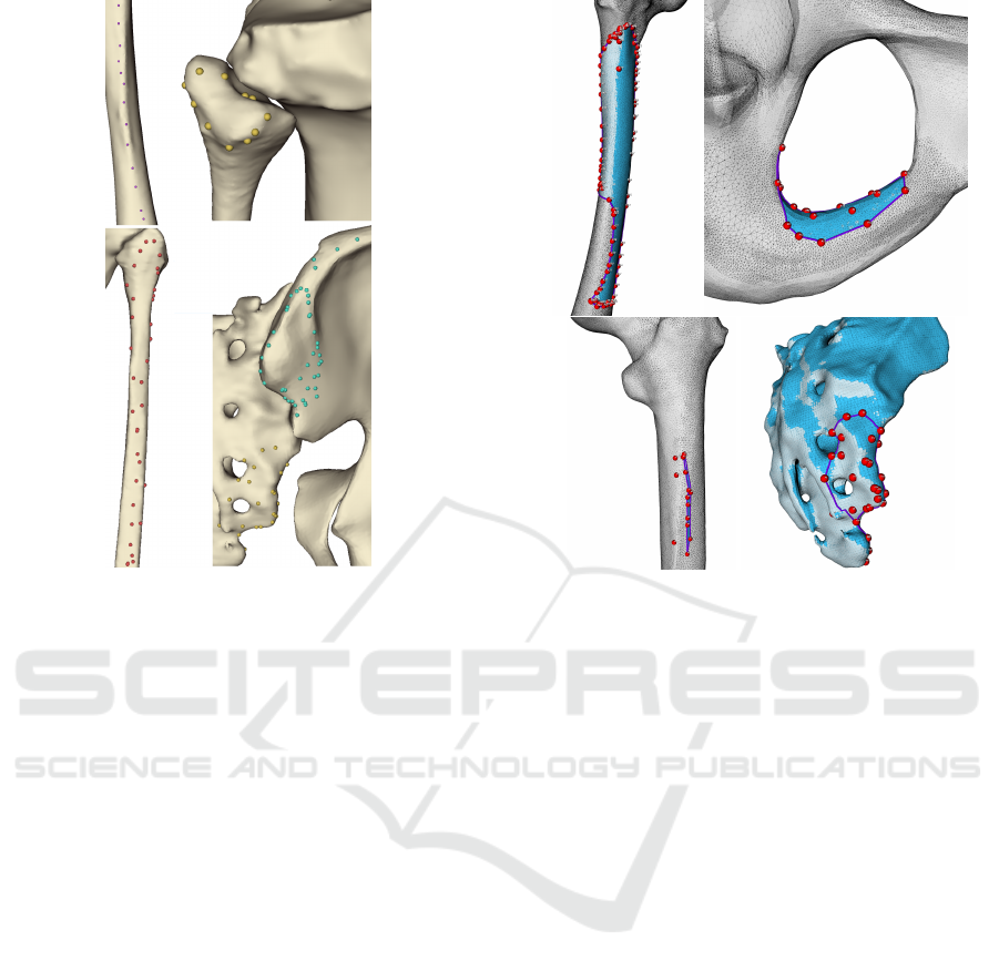
Figure 7: Representative examples of TLEM 2.0 point sets
of muscle attachments. From top to bottom, left to right:
biceps femoris origin, biceps femoris insertion, soleus later-
alis origin, and gluteus maximus superior + inferior origin.
Our samples included all vertices of the bone mesh
triangles plus some points sampled randomly in ev-
ery triangle with an area larger than ε. The num-
ber of samples in such a triangle was determined as
its area divided by ε. In the experiments, we used
ε = π · 0.1 · 0.1, which means our sampling frequency
was about 0.2 mm.
Figure 9 shows the results we obtained. For closed
curves with almost uniform sampling without appar-
ent outliers and noise, represented, e.g., for biceps
femoris insertion, the differences between 2D curve
reconstruction algorithms are negligible. It is also
apparent that only the α-shape algorithm was robust
enough to process every data set. Connect2d, fitcon-
nect, discur, and vicur algorithms could process only
about 70.8% of data sets, stretchdenoise only about
58.3%. The rest failed to process the gluteus medius
posterior insertion, which is not surprising consider-
ing that this data set contains many outliers (see Fig-
ure 10). The poor performance, generally, showed
discur and vicur algorithms.
Further inspection reveals that none of the algo-
rithms could provide acceptable results for the gluteus
maximus inferior insertion and vastus intermedius
origin data sets. In the former case, the reason is
simply that the data contains three outliers outside the
attachment region (probably introduced during an er-
Figure 8: Ground-truth closed curves (purple) for vastus
intermedius origin, obturator externus lateral origin, glu-
teus maximus inferior origin, and gluteus maximus infe-
rior insertion. Surface patches representing the attachment
areas, extracted using the implementation by (Kohout and
Kuka
ˇ
cka, 2014) are shaded in blue.
roneous registration process) – see Figure 10. In the
latter case, the explanation is more complicated. Al-
though the data of vastus intermedius origin seems
quite OK for a human observer (see Figure 8), the
algorithms yield multiple connections between the
points on the left side with those on the right one.
It might be because the sampling frequency on the
boundary is insufficient, and thus the influence of the
single apparent outlier is not negligible. As the fe-
mur bone resembles a cylinder, the geodetics com-
puted for these incorrect edges are not on the same
side, but some lie in the front, others in the back. As a
result, the bone is effectively cut into several parts, as
shown in Figure 10 and, therefore, only a part of the
attachment area is extracted.
On average, the best performance reached α-
shape (72.00%), followed by connect2d (69.35%),
and lenz (67.04%). However, it is needed to point
out that the dice similarity coefficient is not a re-
liable indicator for very narrow attachments repre-
sented by slightly curved lines, for which values as
low as 30% are often visually acceptable. This is
the case of adductor longus insertion, adductor mag-
nus mid insertion, adductor magnus proximal inser-
tion, biceps femoris CB origin, iliopsoas superior in-
GRAPP 2022 - 17th International Conference on Computer Graphics Theory and Applications
240

Muscle attachment
alpha shape
connect2d
hnncrust
fitconnect
stretchdenoise
discur
vicur
crawl
peel
crust
nncrust
ccrust
gathan1
gathang
lenz
adductor magnus distal insertion 94.64% 87.58% 28.79% 92.49% 92.49% 0.48% 14.31% 34.14% 28.37% 24.80% 93.70% 14.57% 26.01% 26.01% 93.38%
adductor magnus mid insertion 78.88% 51.98% 28.83% 28.83% 28.83% 28.83% 28.83% 25.86% 28.83% 28.83% 28.83% 52.22% 28.83% 72.11%
adductor magnus proximal insertion 85.06% 81.97% 24.83% 24.83% 24.83% 24.83% 24.83% 22.88% 24.72% 21.36% 21.36% 21.36% 81.83% 21.36% 86.38%
biceps femoris origin 84.72% 54.63% 19.09% 19.09% 19.09% 19.09% 19.09% 20.48% 19.58% 20.48% 20.48% 20.48% 54.84% 20.48% 26.02%
biceps femoris insertion 98.44% 97.23% 97.23% 97.23% 97.23% 97.23% 97.23% 97.23% 97.23% 97.23% 97.23% 97.23% 97.23% 97.23% 97.95%
gluteus maximus inferior insertion 16.46% 31.96% 28.91% 28.68% 30.09% 27.92% 27.92% 31.64% 35.42% 17.31%
gluteus maximus superior insertion 89.67% 21.92% 33.59% 25.10% 29.46% 91.06% 14.44% 15.27% 18.40% 83.66%
gluteus maximus superior origin 79.92% 87.56% 5.78% 76.52% 76.52% 3.88% 3.55% 94.14% 8.10% 6.89% 81.34% 3.19% 4.26% 7.18% 77.98%
gluteus medius anterior insertion 91.48% 83.15% 7.05% 89.35% 89.35% 16.23% 11.39% 20.65% 12.97% 10.01% 65.61% 14.41% 8.62% 15.88% 84.84%
gluteus medius anterior origin 96.84% 7.22% 13.09% 10.72% 5.59% 93.02% 2.91% 4.24% 5.21% 97.47%
gluteus medius posterior insertion 79.40%
gluteus medius posterior origin 97.31% 98.11% 98.11% 97.98% 97.98% 3.73% 98.08% 98.11% 98.11% 98.11% 98.11% 4.00% 98.11% 98.11% 98.36%
iliopsoas inferior insertion 96.17% 77.17% 8.82% 54.97% 54.97% 0.91% 16.68% 25.79% 17.46% 18.71% 47.84% 11.75% 9.54% 17.81% 95.59%
iliopsoas superior insertion 71.98% 65.20% 49.47% 49.47% 49.47% 49.47% 49.47% 32.39% 32.39% 49.47% 49.47% 49.47% 49.47% 49.47% 66.23%
obturator externus lateral origin 89.09% 62.48% 9.62% 11.78% 5.23% 12.28% 17.84% 10.30% 17.15% 65.52% 7.38% 45.24% 6.08% 78.82%
obturator externus medial origin 97.89% 78.36% 6.40% 80.84% 80.84% 6.48% 4.82% 10.11% 6.14% 6.62% 89.87% 5.68% 1.50% 7.51% 96.77%
sartorius insertion 48.95% 20.88% 61.61% 34.42% 35.86% 74.81% 40.69% 35.02% 48.11% 59.02%
semimembranosus insertion 78.91% 72.93% 34.34% 34.34% 34.34% 34.34% 34.34% 24.14% 34.85% 24.14% 24.14% 24.14% 72.80% 24.14% 78.88%
semimembranosus origin 70.16% 87.90% 12.20% 8.95% 8.95% 1.89% 9.28% 19.69% 12.62% 23.40% 56.29% 8.91% 13.53% 79.03% 73.13%
soleus lateralis origin 71.05% 45.73% 15.31% 15.52% 15.52% 3.64% 7.07% 15.55% 14.89% 11.36% 15.56% 10.60% 51.43% 11.66% 16.24%
soleus medialis origin 15.38% 12.28% 48.25% 46.16% 46.16% 15.54% 47.63% 48.43% 44.07% 45.44% 19.33% 51.41% 12.27% 12.27% 14.24%
vastus intermedius origin 0.06% 6.73% 11.19% 6.42% 10.56% 36.09% 4.49% 22.82% 4.00% 39.64%
vastus medialis inferior origin 36.76% 31.47% 41.63% 42.55% 40.60% 41.45% 41.45% 38.42% 41.45% 33.87%
vastus medialis superior origin 58.85% 34.74% 14.56% 25.18% 20.83% 8.65% 23.99% 13.34% 13.32% 44.78% 12.14% 13.00% 15.50% 53.97%
Figure 9: Dice similarity coefficients of various muscle attachments, obtained for the MDS with different curve reconstruction
algorithms. Missing values mean that the reconstruction algorithm failed. The best performances are marked in bold.
Figure 10: The data sets causing troubles during the pro-
cessing (see the text): gluteus medius posterior insertion
with a lot of internal points (top left), gluteus maximus infe-
rior insertion with three outer points (top right), and vastus
intermedius origin with an insufficient sampling frequency
(bottom). The ground-truth curve is purple, the final con-
tour obtained from α-shape curve is light blue, and geodet-
ics computed from the connectivity found by the lenz algo-
rithm are yellow.
sertion, semimembranosus insertion, soleus medialis
origin, and vastus medialis inferior origin. If we ex-
clude the results of these data sets, we get four al-
gorithms whose performance exceeds 70% on aver-
age: α-shape (78.74%), lenz (76.45%), connect2d
(76.36%), and nncrust (70.05%). Considering that
connect2d failed repeatedly, we can recommend only
α-shape or lenz algorithms for the curve reconstruc-
tion in our context.
For the data sets mentioned above, a better indi-
cator might be the difference in the perimeter of the
reconstructed and ground-truth curves. Table 1 shows
that according to this indicator, the best performing
algorithm is connect2d, with the error of 1.25% on
average but one failure, followed by gathan1 (2.60%
on average), α-shape (3.03%), and lenz (3.43%). All
other algorithms exhibited a worse performance with
multiple failures or average errors exceeding 4% (in
absolute values). We note that median errors were
below 4% in all cases. The order of the five best-
performing algorithms remains the same even when
median errors are considered.
Therefore, it can be concluded that α-shape or
lenz algorithms are universal algorithms suitable for
all cases. This result is also confirmed by a subjec-
tive test, in which a human volunteer assessed all the
reconstructed contours visually, classifying them into
three categories:
• A = no issue or a minor one only without any con-
siderable impact on musculoskeletal modelling,
• B = acceptable but with some issues that might
have some undesirable impacts on musculoskele-
tal modelling, and
• C = unacceptable.
The α-shape and lenz algorithms have almost half
of their contours (48.1% precisely in both cases) in
category A. While hncrust, discur, vicur, peel, crust,
ccrust, gathan1, and gathang algorithms have more
than half of the contours they produced in category
C, α-shape and lenz have there only 4 and 5 contours,
which corresponds to 11.1% and 18.5%, respectively.
Two of these contours belong to gluteus maximus
inferior insertion, and vastus intermedius origin, al-
ready discussed above (see also Figure 10).α-shape
further failed to provide acceptable results for vastus
medialis superior origin, lenz for obturator externus
Non-planar Surface Shape Reconstruction from a Point Cloud in the Context of Muscles Attachments Estimation
241

Table 1: Differences between the perimeters of the reconstructed and ground-truth contours for selected 2D curve reconstruc-
tion algorithms. The best results are bold.
Name α-shape connect2d fitconnect nncrust gathan1 lenz
adductor longus insertion 7.73% 5.82% 7.85% 7.84% 5.82% 8.26%
adductor magnus mid insertion 1.54% 0.00% 1.07% 1.07% 0.00% 0.92%
adductor magnus proximal insertion 2.31% -0.20% 3.79% 3.71% -0.20% 3.11%
biceps femoris origin 1.25% -0.28% 1.37% 0.73% -0.28% 1.41%
iliopsoas superior insertion 6.69% 0.70% 8.35% 8.35% 8.35% 7.05%
semimembranosus insertion 1.85% -0.04% 2.48% 2.68% -0.04% 1.97%
soleus medialis origin -1.31% -2.98% -5.75% -0.22% -2.99% -0.84%
vastus medialis inferior origo 1.59% 7.63% 3.09% 3.86%
Avg(abs(error)) 3.03% 1.25% 3.83% 4.03% 2.60% 3.43%
lateral origin, soleus lateralis origin, and soleus medi-
alis origin. In all four cases, the attachments are much
more stretched in one dimension than in the other.
Due to sparse sampling, the MDS increased further
this ratio, producing points visually lying almost on
a one-dimensional object (see Figure 11). All algo-
rithms then struggled with such data.
Figure 11: Soleus lateralis origin after being transformed
into 2D using projection onto the best fit plane (left) and
using the multidimensional scaling technique (right).
We, therefore, compared the results with those ob-
tained when the input points were projected onto the
plane fitted to the data by the least-squares method
instead of using the multidimensional scaling tech-
nique. Table 2 show that although some algorithms
benefit from the MDS technique (e.g., fitconnect,
stretchdenoise, or peel), others, without any doubt,
perform better without it (e.g., lenz or nncrust). As
for the subjective tests, lenz algorithm came in first
with 15 (i.e., 55.6%) muscle attachments in category
A, 11 (i.e., 40.7%) in category B and only vastus
intermedius origin in category C. The second place
was taken by α-shape with 10 (i.e., 37%) muscle at-
tachments in category A, 13 (i.e., 48.1%) in category
B, and 4 (i.e., 14.8%) in category C. Clearly, while
α-shape achieved more acceptable results with the
MDS, lenz demonstrated different behaviour.
However, we must point out that a projection of
points onto a common plane is not suitable when the
curve to be reconstructed bends several times, e.g.,
like in the case of a narrow saddle. Although such
cases are pretty rare in the context of muscle attach-
ments, they seem to be frequent in the aneurysm neck
identification problem.
Table 2: Difference of the average performance when using
the MDS and when using the projection onto a common
plane. Positive values mean that the MDS outperforms the
projection. Dice similarity coefficients (DSC) are used as
a performance indicator for the data for which DSC is a
reliable indicator (see the text for explanation). For the rest,
errors in the muscle attachments perimeters (PER) are used.
Algorithm DSC PER
α-shape -0.37% -0.31%
connect2d -8.80% 0.23%
hnncrust 8.83% 0.00%
fitconnect 11.54% 0.25%
stretchdenoise 17.10% -0.26%
discur -8.46% 6.38%
vicur -5.70% -0.01%
crawl -6.69% -0.03%
peel 9.61% 0.05%
crust 4.31% -0.08%
nncrust -6.63% -0.57%
ccrust -0.17% -6.31%
gathan1 3.87% -2.11%
gathang -12.59% -11.09%
lenz -12.66% -0.72%
We also did some preliminary testing of the RBF
approach for ordering the vertices and smoothing the
curve. The primary purpose of this test is to check
whether the RBF approach will be capable of creating
a closed and non-self-intersecting curve in 2D.
If the outliers or apparent nonuniformity are
present, the resulting curve is far from expectations
(e.g. vastus intermedius origin on the left of Fig-
ure 12). Luckily, this approach gives better results
for many other attachment areas (e.g. gluteus medius
posterior on the right of the Figure 12). The polar
coordinate system for the dimension reduction causes
problems in some cases, mainly if there is a wide an-
gle without any vertex (left image of the Figure 12,
bottom part), causing a single or even multiple self-
intersectional loops. Approximating the curve instead
of interpolating may solve these issues.
GRAPP 2022 - 17th International Conference on Computer Graphics Theory and Applications
242

Figure 12: Two radial basis function approximation results.
Vastus intermedius origin is on the left. The connection be-
tween both ends of the attachment area does not turned out
well due to looping the curve. Gluteus medius posterior
origin is on the right. The shape is approximated by expec-
tations.
5 CONCLUSION AND FUTURE
WORK
This paper investigated the options of reconstructing
a closed space curve from the points sampled on that
curve, supporting sparse sampling and noisy data with
multiple outliers. Our extensive experiments, per-
formed on the TLEM 2.0 data sets (Carbone et al.,
2015) in the context of muscle attachments estima-
tion, lead us to the following recommendations. If
the curve to be reconstructed is not expected to have
a shape of a narrow saddle or be otherwise strangely
bent, the points should be projected onto the plane
that best fit the input data. The lenz algorithm (Lenz,
2006) should be used on the projected points to find
the primary connectivity between the input points.
Suppose this algorithm is unavailable or the expec-
tations on the curve shape do not hold. In that case,
the input data should be transformed onto the plane
using the multidimensional scaling (MDS) technique
(Cox and Cox, 2008). The α-shape algorithm (Edels-
brunner et al., 1983) should be then used on the trans-
formed points (instead of the lenz algorithm), with the
disc radius being slightly above half of the maximal
shortest distance between pairs of transformed points.
If neither algorithm is available, connect2d or nncrust
(see (Ohrhallinger et al., 2021)) are a decent choice.
Providing that the surface on which the space
curve lies is available, the reconstructed curve can
be refined by tracing the shortest paths between each
pair of points connected by an edge. A non-manifold
curve, i.e., a curve containing vertices of valence
larger than 2, can be converted into a manifold one
using the algorithm proposed in the paper, based on
iso-contour extraction from a scalar field describing
for each point on the surface its distance to the curve.
If the object bounded by the curve covers only a tiny
portion of the surface in any direction or the surface
is open, this conversion is reliable.
REFERENCES
Berger, M., Tagliasacchi, A., Seversky, L. M., Alliez, P.,
Guennebaud, G., Levine, J. A., Sharf, A., and Silva,
C. T. (2016). A survey of surface reconstruction from
point clouds. Computer Graphics Forum, 36(1):301–
329.
Carbone, V., Fluit, R., Pellikaan, P., van der Krogt, M.,
Janssen, D., Damsgaard, M., Vigneron, L., Feilkas,
T., Koopman, H., and Verdonschot, N. (2015). TLEM
2.0 – a comprehensive musculoskeletal geometry
dataset for subject-specific modeling of lower extrem-
ity. Journal of Biomechanics, 48(5):734–741.
Carr, J. C., Beatson, R. K., Cherrie, J. B., Mitchell, T. J.,
Fright, W. R., McCallum, B. C., and Evans, T. R.
(2001). Reconstruction and representation of 3d ob-
jects with radial basis functions. In Proceedings of the
28th annual conference on Computer graphics and in-
teractive techniques. ACM Press.
Cervenka, M., Smolik, M., and Skala, V. (2019). A new
strategy for scattered data approximation using radial
basis functions respecting points of inflection. Com-
putational Science and Its Applications.
Cox, M. A. A. and Cox, T. F. (2008). Multidimensional
scaling. In Handbook of Data Visualization, pages
315–347. Springer Berlin Heidelberg.
Edelsbrunner, H., Kirkpatrick, D., and Seidel, R. (1983).
On the shape of a set of points in the plane. Informa-
tion Theory, IEEE Transactions on, 29:551 – 559.
Fukuda, N., Otake, Y., Takao, M., Yokota, F., Ogawa, T.,
Uemura, K., Nakaya, R., Tamura, K., Grupp, R. B.,
Farvardin, A., Armand, M., Sugano, N., and Sato, Y.
(2017). Estimation of attachment regions of hip mus-
cles in CT image using muscle attachment probabilis-
tic atlas constructed from measurements in eight ca-
davers. Int J Comput Assist Radiol Surg., 12(5):733–
742.
Kohout, J. and Kuka
ˇ
cka, M. (2014). Real-time modelling of
fibrous muscle. Computer Graphics Forum, 33(8):1–
15.
Krishnan, K. (2013). Geodesic computations on surfaces.
The VTK Journal.
Lenz, T. (2006). How to sample and reconstruct curves
with unusual features. In Proceedings of the 22nd
European Workshop on Computational Geometry
(EWCG), pages 29–32.
Ohrhallinger, S., Peethambaran, J., Parakkat, A. D., Dey,
T. K., and Muthuganapathy, R. (2021). 2d points
curve reconstruction survey and benchmark. Com-
puter Graphics Forum, 40(2):611–632.
Peyr
´
e, G. (2009). Geodesic methods in computer vision
and graphics. Foundations and Trends® in Computer
Graphics and Vision, 5(3-4):197–397.
Skala, V. and Cervenka, M. (2020). Novel rbf approxima-
tion method based on geometrical properties for sig-
nal processing with a new rbf function: Experimental
comparison. 2019 IEEE 15th International Scientific
Conference on Informatics.
Non-planar Surface Shape Reconstruction from a Point Cloud in the Context of Muscles Attachments Estimation
243
