Classiﬁcation Performance of RanSaC Algorithms

with Automatic Threshold Estimation

ement Riu

, Vincent Nozick

, Pascal Monasse

and Joachim Dehais

Universit

e Paris-Est, LIGM (UMR CNRS 8049), UGE, ENPC, F-77455 Marne-la-Vall

ee, France

Arcondis AG 4153 Basel, Switzerland

Keywords:

Multi-View Stereo, Structue-from-Motion, RanSaC, Semi-synthetic Dataset, Benchmark.

Abstract:

The RANdom SAmpling Consensus method (RanSaC) is a staple of computer vision systems and offers a

simple way of ﬁtting parameterized models to data corrupted by outliers. It builds many models from small

sets of randomly selected data points, and then scores them to keep the best. The original scoring function is

the number of inliers, points that ﬁt the model up to some tolerance. The threshold that separates inliers from

outliers is data- and model-dependent, and estimating the quality of a RanSaC method is difﬁcult as ground

truth data is scarce or not quite reliable. To remedy that, we propose a data generation method to create at will

ground truths both realistic and perfectly reliable. We then compare the RanSaC methods that simultaneously

ﬁt a model and estimate an appropriate threshold. We measure their classiﬁcation performance on those semi-

synthetic feature correspondence pairs for homography, fundamental, and essential matrices. Whereas the

reviewed methods perform on par with the RanSaC baseline for standard cases, they do better in difﬁcult

cases, maintaining over 80 % precision and recall. The performance increase comes at the cost of running

time and analytical complexity, and unexpected failures for some algorithms.

1 INTRODUCTION

Over fourty years have passed since the publication of

the RANdom SAmple Consensus algorithm (Fischler

and Bolles, 1981). The algorithm approximates a so-

lution to the NP-hard consensus maximization prob-

lem (Chin et al., 2018): ﬁtting a parameterized model

to data corrupted by noise and outliers. RanSaC gen-

erates tentative models using random, minimal sub-

sets of data and validates them with the distance of

data points to each model. Data points whose model

distance are below a given threshold are inliers, and

the retained model maximizes the inlier count, or

consensus. Deﬁning this threshold however requires

knowing the noise level in the data. Some methods lift

this constraint by estimating jointly a threshold and a

model. For them, the inlier count is replaced by new

measures involving both threshold and inlier count for

optimization. We call these methods adaptive or au-

tomatic.

We review these methods and examine their per-

formance on a benchmark of three computer vi-

sion problems central to Multi-View Stereo (MVS)

and Structure-From-Motion (SfM) pipelines (Schon-

berger and Frahm, 2016; Moulon et al., 2016): ho-

mography, fundamental and essential matrix ﬁtting.

Data for these problems consists of feature point pair

correspondences, leading the algorithm to classify

them as inlier or outlier.

Firstly, automatic threshold estimation does ben-

eﬁt MVS pipelines (Moulon et al., 2012), although

its performance should be measured on ground-truth

data independently. Secondly, incremental MVS

pipelines also beneﬁt from good inlier classiﬁcation,

as inliers are triangulated to from 3D points, there-

after used as anchors for following views to estimate

their pose through Perspective from n Points (PnP).

Thirdly, since RanSaC methods are the basis of SfM

and MVS software, robust analysis will improve the

state of the art. Fourthly and ﬁnally, deep-learning 3D

pipelines use the output of MVS pipelines, most often

(Schonberger and Frahm, 2016), for training database

generation (Li and Snavely, 2018).

We ﬁrst contribute a method to create semi-

synthetic data with ground truth labels to assess clas-

siﬁcation power of RanSaC algorithms. Previous

artiﬁcial datasets are unrealistic; e.g. (Cohen and

Zach, 2015) performs the evaluation on plane es-

timation in random 3D point clouds, and (Barath

et al., 2019) generates random homographies and cor-

Riu, C., Nozick, V., Monasse, P. and Dehais, J.

Classiﬁcation Performance of RanSaC Algorithms with Automatic Threshold Estimation.

DOI: 10.5220/0010873300003124

In Proceedings of the 17th International Joint Conference on Computer Vision, Imaging and Computer Graphics Theory and Applications (VISIGRAPP 2022) - Volume 5: VISAPP, pages

723-733

ISBN: 978-989-758-555-5; ISSN: 2184-4321

723

Table 1: Notations.

Deﬁnition Description

k ∈ N

dimension of data points

S = R

space of data points

P ⊂ S set of input data points

d ∈ N

degrees of freedom of a model

Θ ⊂ R

space of model parameters

θ ∈ Θ parameter vector of a model

s ∈ N

data sample size

Sa : 2

→ S

sampling function

F : S

→ Θ ﬁtting function

p : [0,1] → [0,1] proba. of sampling inliers only

D : S × Θ → R point-model residual function

σ ∈ R inlier threshold

I : Θ × R → 2

inlier selector function

I = I(θ,σ) ⊂ P

set of model inliers

Q : 2

× Θ → R model quality function

respondences. Real datasets on the opposite end can-

not offer a control over the noise and outliers: they

often rely on an algorithm to calibrate an active sen-

sor to the data which introduces error like the KITTI

dataset (Geiger et al., 2012) and the 7 scenes dataset

(Shotton et al., 2013) or do not correct inlier noise as

in (Cordts et al., 2016). Our method offers the pos-

sibility to create, from any image dataset, a realistic

semi-synthetic dataset.

Note that there have already been comparative

studies of RanSaC, such as (Choi et al., 2009).

These studies however focus on threshold-controlled

RanSaC derivatives on a small real-world dataset

without ground truth. We contribute an analysis

of the classiﬁcation and retrieval power of adaptive

RanSaC algorithms. We thus pit threshold-free meth-

ods against each other, rather than against baseline

RanSaC as was done before.

Section 2 reviews the automatic RanSaC meth-

ods, Section 3 the benchmark data and methods. Sec-

tions 4 and 5 cover the results and their analysis, and

Section 6 concludes.

2 AUTOMATIC RanSaC

METHODS

2.1 Notation

We reuse and simplify the notation of (Barath et al.,

2019), standardized in Table 1. Input points exist in

S = R

,k > 0, with the input point set noted as P ⊂ S.

For image coordinates, the point dimension k = 2; for

pair correspondences, k = 4.

A model of d degrees of freedom exists in Θ ⊂ R

and can be obtained via the ﬁtting function F, applied

to a set of data points sampled by the sampling func-

tion Sa. d = 8 for homographies, 7 for fundamental

matrices, and 5 for essential matrices.

The probability of Sa drawing an uncontaminated

sample (including only correct data) is p(ε), with ε ∈

[0,1] the true (hence generally unknown) inlier ratio.

Sa typically samples s points uniformly in P , hence

p(ε) = ε

, an increasing function of ε.

Given a model θ, we can calculate the residual

error between that model and a data point P using

D(P,θ). I selects the points that are inliers to a model

based on the residuals. Finally, Q deﬁnes the quality

of the ﬁt θ on P .

While D is model-dependent, the standard selec-

tor I keeps points with residuals below a threshold σ:

I = I(θ,σ) = {P ∈ P : D(P,θ) < σ}. Q(I , θ) = |I |

is then the number of inliers. Since inlier count in-

creases with σ, standard Q deﬁnitions are unreliable

quality measures for RanSaC variants. Algorithm 1 is

the pseudo-code for a generic RanSaC. A type II error

corresponds to missing the true model due to insufﬁ-

cient search.

Input: P , Sa, F, p, Q, σ

Input: conﬁdence against type II error β,

max

(or min. inlier rate ε)

Output: Best model parameters and set of

inliers

max

0, q

max

= 0

it = 0 (and it

max

ln(1−β)

ln(1−p(ε))

if ε is input)

while it ≤ it

max

sample = Sa(P ), θ = F(sample)

I = I(θ,σ), q = Q(I ,θ)

if q > q

max

then

max

= q,θ

max

= θ,I

max

= I

ε = |I |/|P |,it

max

ln(1−β)

ln(1−p(ε))

it = it + 1

return θ

max

Algorithm 1: RanSaC algorithm.

2.2 Existing Algorithms

The methods gathered in Table 2 generate new in-

lier and model quality deﬁnitions to behave adap-

tively. They rely on three types of consistency mod-

els: inlier, outlier, and cross-model. An inlier- (resp.

outlier-)consistent method enforces a parameterized

distribution on the inlier (resp. outlier) residuals, and

searches for a model and parameter set that ﬁt the

data. A cross-model-consistent method looks for re-

peated patterns in residuals of different models us-

ing cross correlations or clustering. The original

RanSaC (Fischler and Bolles, 1981) algorithm uses

VISAPP 2022 - 17th International Conference on Computer Vision Theory and Applications

724

Table 2: Overview of robust ﬁtting methods with adaptive inlier criteria. Bracketed terms in the “Consistency assumption”

column specify where the assumption is made.

Ref. Consistency assumption Optimized function

(Fischler and Bolles, 1981) Bounded residuals (inliers) Inlier set size

(Miller and Stewart, 1996) Gaussian residual distribution (inliers) Scale estimate

(Wang and Suter, 2004) Gaussian (inliers) Inlier/threshold

Minimal residual density (transition)

(Fan and Pylv

ainen, 2008) Gaussian (inliers) Scale estimate

Residuals correlate (cross-model)

(Choi and Medioni, 2009) Low parameter variance (cross-model) Variance

(Moisan et al., 2012) Problem speciﬁc (outlier) Number of false alarms

(Cohen and Zach, 2015) Uniform (outliers) Likelihood

(Moisan et al., 2016) Problem speciﬁc (outliers) Number of false alarms

(Dehais et al., 2017) Data-driven (outliers) False discovery rate

(Barath et al., 2019) Uniform (inliers) - Uniform (outliers) Deviation

(Rabin et al., 2010) Problem speciﬁc (outliers) Greedy number of false alarms

(Isack and Boykov, 2012) Graph cuts energy

(Toldo and Fusiello, 2013) Residuals correlate (cross-model) Inlier cluster merging cost

(Magri and Fusiello, 2014) Residuals correlate (cross-model) Residual cluster merging cost

(Magri and Fusiello, 2015) Residuals correlate (cross-model) Factorization error of residual matrix

inlier consistency: all inliers have residuals below a

certain threshold.

The ﬁrst automatic threshold method was

MUSE (Miller and Stewart, 1996). MUSE assumes

that inlier residuals follow a Gaussian distribution,

and estimates the noise level for all inlier sets of all

tested models. The smallest noise for each model

becomes its quality measure, and the model with the

smallest noise level is selected overall.

(Wang and Suter, 2004) relies on inliers follow-

ing a unimodal distribution (speciﬁcally Gaussian in

experiments). For single models, this method puts a

threshold on residual distribution density. The quality

measure is the ratio of inliers to inlier threshold value.

The method in (Fan and Pylv

ainen, 2008)

merges inlier and cross-model consistency. This

method uses the weighted median absolute deviation

of all residuals as both scale estimate and quality

function. Each time a data point has a small resid-

ual for a sampled model, its weight and probability to

be sampled increase. This way, the weight biases the

quality function towards the median absolute devia-

tion of inliers to stable models.

StarSaC (Choi and Medioni, 2009) uses cross-

model consistency as well, namely that variance of

model parameters is minimal for the optimal thresh-

old. The method calls RanSaC with multiple thresh-

olds, multiple times per threshold. The quality mea-

sure is the variance of resulting model parameters for

a given threshold.

A Contrario RanSaC (Moisan et al., 2012;

Moisan et al., 2016) (AC-RanSaC, originally named

ORSA (Moisan and Stival, 2004)) was the ﬁrst

outlier-consistent method. AC-RanSaC approximates

for each problem the probability distribution of resid-

uals for random input: the background distribution.

It then minimizes a combinatorial prediction of false

inliers by comparing the cumulative distributions of

data and background residuals.

An extension of AC-RanSaC (Dehais et al., 2017)

adapts the method in two ways: by generating out-

lier data from inlier data, and simplifying the signiﬁ-

cance measure. This method scrambles input matches

to generate background distributions, and seeks the

model with the most inliers subject to a maximal rate

of inliers in the background data.

The likelihood-ratio method (Cohen and Zach,

2015) relies on a uniform distribution of outlier resid-

uals. The quality function approximates the likeli-

hood of each model against this uniform distribution,

using substantial statistical derivations.

MAGSAC (Barath et al., 2019) is the most recent

publication on this work’s subject. It combines in-

lier and outlier consistency assumptions, where both

follow uniform distributions on different intervals.

MAGSAC then estimates the model’s deviation from

the background noise, without explicitly classifying

inputs into inliers and outliers.

Other methods exist to detect multiple models in

data; though they are out of scope, we list some here.

(Rabin et al., 2010) uses the principle of A Contrario

RanSac (Moisan et al., 2012) in a greedy optimization

to extract multiple models. (Isack and Boykov, 2012)

generates multiple models, before attaching data to

those models to minimize total residuals and number

of models. J-Linkage (Toldo and Fusiello, 2013), its

Classiﬁcation Performance of RanSaC Algorithms with Automatic Threshold Estimation

725

extension T-Linkage (Magri and Fusiello, 2014), and

Low-Rank Preference Analysis (Magri and Fusiello,

2015) rely on cross-model consistency, while using

different methods to cluster inlier sets and models

jointly.

3 BENCHMARK

3.1 Data Generator

The distributions of inliers and ouliers in the image

space have a major impact on the effectiveness of

model ﬁtting. Benchmarks on data extracted from

photographs are invaluable, but lack the power to gen-

eralize observations because of their small size and

the lack of control over noise and outliers. Synthetic

data on the other hand are ﬂexible and customizable

but unrealistic as the chosen model generation and in-

lier sampling methods impact the results.

We propose a simple procedure to generate real-

istic, semi-synthetic data with ground truth classiﬁca-

tion. It gives access to real models and inliers, with

outliers whose distance to the model is controlled.

The data generator takes an image pair with point

matches and evaluates its underlying model using

AC-RanSaC (Moisan et al., 2012; Moisan et al.,

2016) at arbitrary precision and up to 10 000 itera-

tions. The returned model is then used as “ground

truth”, and the estimated inliers as the basis for data-

driven yet perfect inliers.

To generate perfect inliers, the matches are mod-

iﬁed with respect to the ground truth model. For

homographies, inlier points in the ﬁrst image are

mapped into the second using the ground truth ho-

mography (ﬁgure 1). For fundamental and essential

matrices, the point on the second image of each inlier

match is projected on the true epipolar line of the ﬁrst

point (ﬁgure 2).

The artiﬁcial inlier matches and outlier matches

can then be derived from those “ground truth” inlier

matches. Inlier matches are created by adding noise

uniformly drawn in [−σ

noise

,σ

noise

]

to the second im-

age point of each match to generate a controled pixel

error. Uniform noise gives here better control and

testability for the inlier/outlier threshold than Gaus-

sian noise, which is unbounded.

Once inlier matches are generated, outliers are in-

serted by generating random matches in the two im-

ages, uniformly sampled in error space ensuring a dis-

tance to the model greater than the maximum inlier

error σ

noise

. Sampling in error space is explained for

homography estimation in ﬁgure 3 and for fundamen-

tal and essential matrix estimation in ﬁgure 4. This

choice of distribution in error space returns a realis-

tic outlier distribution and truly challenges the algo-

rithms. A simple uniform distribution of outliers in

match space on the contrary has too little structure

to disturb the RanSaC algorithm. For each dataset

and inlier ratio, we generate enough outliers to ob-

tain the desired ratio, and downsample uniformly to

have 4000 data points or fewer.

3.2 Tested Algorithms

We benchmark seven algorithms with varied ap-

proaches to inlier classiﬁcation: the baseline RanSaC

(Fischler and Bolles, 1981), MUSE (Miller and Stew-

art, 1996), StaRSaC (Choi and Medioni, 2009),

A-Contrario RanSaC (AC-RanSaC) (Moisan et al.,

2016), Likelihood Ratio Test (LRT) (Cohen and Zach,

2015), Marginalizing Sample Consensus (MAGSAC)

(Barath et al., 2019) and Fast-AC-RanSaC—an adap-

tation of AC-RanSaC. (Isack and Boykov, 2012;

Toldo and Fusiello, 2013; Magri and Fusiello, 2014),

though relatively recent, have been excluded as they

tackle the multi-model settup which we do not con-

sider in this study.

RanSaC acts as baseline, with ﬁxed inlier/outlier

thresholds σ(px) to show non-adaptive results. To

avoid degenerate cases in the worst case we

strengthen its stopping criterion to ensure it draws

5 outlier-free samples instead of just 1 with conﬁ-

dence β. This requires a modiﬁcation in the formula

for it

max

in Algorithm 1.

MUSE proposes an improvement over Least Me-

dian of Squares (Leroy and Rousseeuw, 1987) with

a new objective function based on a scale estimate

to increase robustness wrt outliers. The algorithm

works similarly to RanSaC, with multiple iterations

of a minimal sampler estimating a model and then

ranking based on their scale estimate. We adapted the

algorithm by adding the classic termination criterion

of RanSaC to speed up the execution.

StaRSaC removes the need for a user set threshold

of RanSaC by launching multiple RanSaCs for differ-

ent thresholds. It then estimates at each threshold the

variance over the parameters and the threshold yield-

ing the lowest variance is selected. Our implemen-

tation uses the same thresholds as (Cohen and Zach,

2015) to speed up the process by only considering

thresholds that make sense in pixel-scale problems.

AC-RanSaC seeks the model with the lowest risk

of type I error. This is measured as the Number of

False Alarms (NFA), which estimates the expected

number of false positive models generated by an in-

VISAPP 2022 - 17th International Conference on Computer Vision Theory and Applications

726

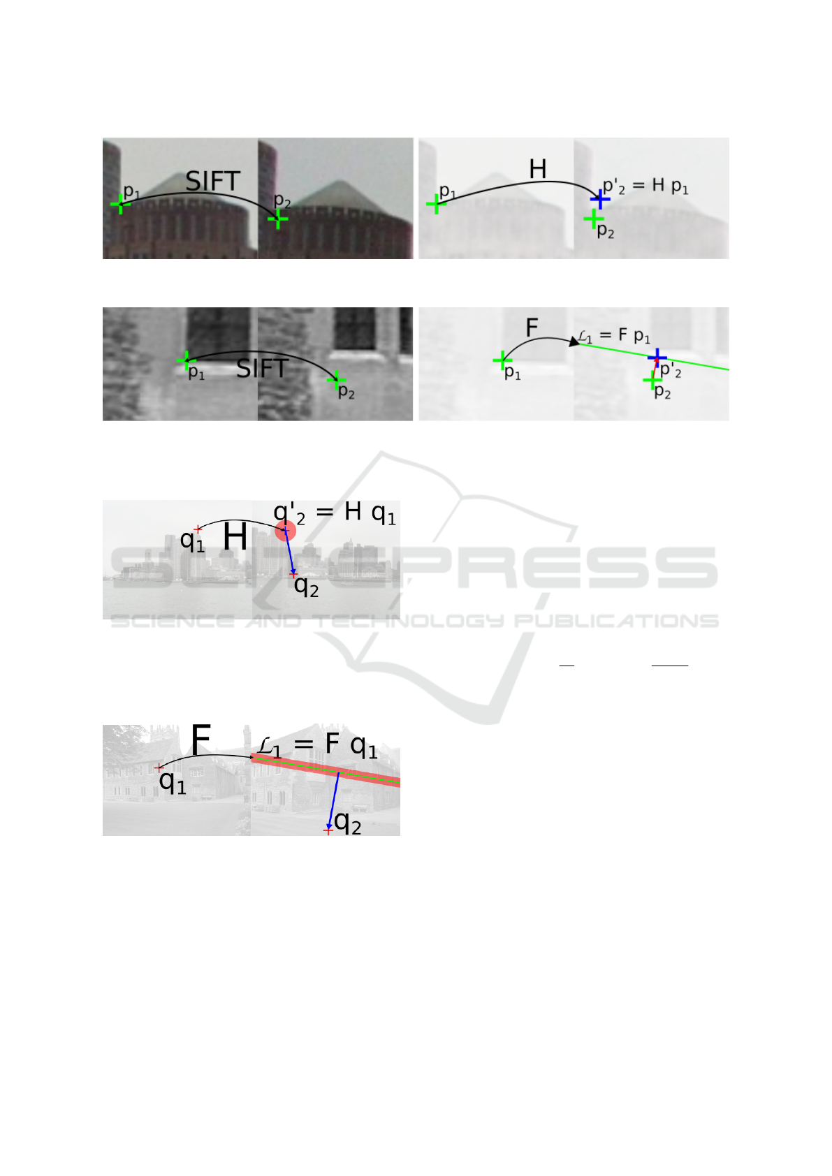
Figure 1: From an imperfect match (p

, p

) considered inlier by AC-RanSaC, the “perfect match” (p

, p

) is constructed

such that p

= H p

using a realistic homography H given by AC-RanSaC.

Figure 2: From an imperfect match (p

, p

) considered inlier by AC-RanSaC, the “perfect match” (p

, p

) is constructed

using p

the orthogonal projection of p

on the epipolar line L

= F p

where F is a realistic fundamental matrix given by

AC-RanSac. This does not guarantee that p

represents the same physical point as p

, but that some 3D point at possibly

different depth projects exactly at p

and p

Figure 3: A random point q

is drawn from the left image.

Using the ground truth model H, its perfect match q

= Hq

is computed. Then a direction and a distance to q

are drawn

uniformly in order to create q

so that it remains in the im-

age and out of the inlier zone (marked in red) deﬁned by the

inlier noise level.

Figure 4: A random point q

is drawn from the left image.

Using the ground truth model F, the epipolar line L

= Fq

is computed. Then position on this line and a distance to

are drawn uniformly in order to create q

so that it re-

mains in the image and out of the inlier zone (marked in

red) deﬁned by the inlier noise level.

lier set:

NFA(θ,σ) ∼



|P |

k(σ)



k(σ)



k(σ)−s

, (1)

with k(σ) = |I(θ,σ)| the number of inliers at thresh-

old σ and p

the relative area of the image zone

deﬁnining inliers at σ. This function is computed

for all σ ≤ σ

max

such that k(σ) ∈ {s + 1,..., n}. The

method is virtually parameter-free, with σ

max

= +∞

and the NFA upper bound NFA

max

= 1.

The Likelihood Ratio Test (LRT) proposes a fast

method to control type I and type II errors. Its qual-

ity function is the likelihood that the dataset is non-

random for a given model:

L(ε,σ) = 2|P |



εlog

+ (1 − ε)log

1 − ε

1 − p



, (2)

with inlier ratio ε = k(σ)/|P | and σ spanning a prede-

ﬁned list {σ

min

,. . . , σ

max

}. The adjustment of it

max

the same as RanSaC, with an early bailout system to

sift through models faster, controlled by a new param-

eter γ for the type II error (rejection of a good model).

MAGSAC introduces a new quality function,

based on the likelihood of a model given uniform in-

liers and outliers, a speedup method using computing

blocks, and a post processing method, σ-consensus,

that reﬁts the ﬁnal model on a weighted set of pseudo-

inliers. It uses four parameters: the threshold for

pseudo-inliers σ

max

, a reference threshold σ

re f

, a

lower bound on model likelihood, and the number of

data blocks.

Fast-AC-RanSaC is a speed up of AC-RanSaC by

exploiting ideas from LRT. The idea to create this

method comes from our observations, see Section 5.

It uses the same objective function as AC-RanSaC but

instead of testing all thresholds it considers the same

quantiﬁed thresholds as LRT. Using this selection of

Classiﬁcation Performance of RanSaC Algorithms with Automatic Threshold Estimation

727

thresholds removes the need for a sorting of the resid-

uals and thus speeds up the method.

3.3 Performance Measures

To compare the classiﬁcation power of the various al-

gorithms, we use precision—the ratio of correctly de-

tected inliers among all detected inliers—and recall—

the ratio of correctly detected inliers among true in-

liers. To represent results more easily, we use the har-

monic mean of precision and recall, the F1-Score. We

quantify the impact of noise and outliers on these met-

rics using the semi-synthetic data of Section 3.1. For

efﬁciency evaluation, we measure execution time.

As MAGSAC does not separate data points into

inliers and outliers but weighs them, we evaluate

its performance through three metrics: highest re-

call at the precision of AC-RanSaC, which will be

called Magsac-P, highest precision at the recall of

AC-RanSaC, Magsac-R, and weighted equivalents of

precision and recall, Magsac-W.

3.4 Parameters

We experimented the data generator on the

SIFT (Lowe, 2004) point matches from the USAC

dataset as well as SIFT points computed on Multi-H,

kusvod2 and the homogr datasets. A SIFT ratio of

0.6 was used. USAC (Raguram et al., 2012) proposes

SIFT matches for 10 homography image pairs, 11

fundamental matrix image pairs, and 6 essential

matrix image pairs with calibration matrices. Multi-

H (Barath et al., 2016) proposes 24 fundamental

matrix image pairs, kusvod2 16 fundamental matrix

image pairs, and homogr 16 homography image

pairs.

The inlier noise σ

noise

varied between 0 and 3 pix-

els by steps of 0.1. The outlier ratio 1 − ε varied be-

tween 0 and 0.9 by steps of 0.1. For each image pair

and setting, we generate N

gen

= 5 different datasets,

and run each algorithm N

run

= 5 times on each for

a total of 25 experiments. We average the precision

and recall over each dataset and run, excluding cases

where an algorithm failed to ﬁnd a good model.

As minimal solvers F, we use the standard 4-point

algorithm for homography and 7-point algorithm for

fundamental matrix (Hartley and Zisserman, 2004),

and the 5-point algorithm for essential matrix (Nist

er,

2004).

We take the standard RanSaC algorithm as base-

line and benchmark MUSE, StarSAC, LRT, AC-

RanSaC, Fast-AC-RanSaC, and MAGSAC algo-

rithms. RanSaC and AC-RanSaC implementations

http://cmp.felk.cvut.cz/data/geometry2view/

came from (Moulon, 2012), MAGSAC from (Barath,

2019), MUSE from VXL

whereas LRT, Fast-

AC-RanSaC and StarSAC were implemented from

scratch.

The parameters deﬁned in section 3.2 are set as

follows (from the relevant publicaion when avail-

able). β, the standard success conﬁdence, is set to

0.99. σ

max

, the inlier search cutoff threshold for AC-

RanSaC, Fast-AC-RanSaC, StarSaC and LRT, is set to

16 pixels to improve speed. NFA

max

, the NFA thresh-

old for AC-RanSaC and Fast-AC-RanSaC, is set to 1

false alarm. The other parameters of LRT, were set to

α = 0.01, γ = 0.05.

The other parameters of MAGSAC were set to p =

10 data partitions, σ

max

= 10 pixels, and σ

re f

= 1.

4 RESULTS

Before presenting results for the different methods,

StarSAC has been excluded from this benchmark. In-

deed, after initial tests, it runs very slowly, even with

modiﬁcation to the initial algorithm to reduce run-

time. A usual run will take 3 to 5 minutes with preci-

sion and recall only slightly above baseline.

Figure 5 gives an overview of each algorithm’s

execution time. LRT, MUSE, Fast-AC-RanSaC and

RanSaC are usually the fastest, with LRT faster than

the others on easy cases. Both LRT and RanSaC how-

ever are quite sensitive to the task complexity: when

facing high inlier noise or outlier ratio, their runtime

increases signiﬁcantly, sometimes up to four or ﬁve

seconds per run. MUSE and Fast-AC-RanSaC keep

relatively low runtimes in all settings, always below

1s. AC-RanSaC’s runtime is not impacted by inlier

noise, only by the number of matches in the dataset.

Its runtime remains almost always under one second

per run, though it is often the slowest algorithm on

easy settings. However, it can be faster than Fast-AC-

RanSac on easy settings with not many points where

the sorting time of residuals is fast compared to the

computation of the residuals themselves. MAGSAC

is the most efﬁcient algorithm on complex tasks with

runtimes up to ten times lower than AC-RanSaC.

However, because of instabilities in MAGSAC’s exe-

cution, a 1-second cap was used: for inlier noise level

above 1 pixel or outlier ratio below 0.4, MAGSAC

can ﬁnd a good model but still fail to terminate.

Except for RanSaC, no algorithm presented a

compromise between precision and recall (one in-

creasing while the other decreases). This justiﬁes the

use of F1-Score over either precision or recall.

https://github.com/vxl/vxl

VISAPP 2022 - 17th International Conference on Computer Vision Theory and Applications

728

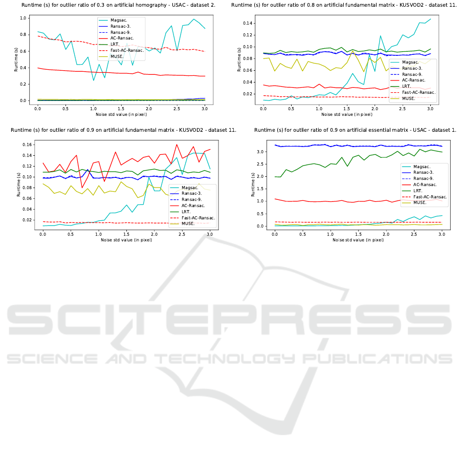
Figure 5: Runtimes over different inlier noise levels and outlier ratios. The ﬁtting problem, dataset name, and image pair

number are in each graph title. Ransac-σ corresponds to RanSaC with threshold σ.

Trends in behavior were impacted by the noise

level and outlier ratio for all algorithms, but were nei-

ther by task, be it homography, fundamental matrix

or essential matrix estimation, nor by dataset. While

performance differed between image pairs or different

tasks, performance always decreased consistently rel-

ative to the data generator parameters. Figures 6 and

7 illustrate the typical behaviors with low and high

outlier ratios on a variety of estimation problems and

datasets. An intermediate setting, for example an out-

lier ratio around 0.5, is not included as the behavior

was observed to be intermediate between the two ex-

tremes.

The two ﬁxed-threshold RanSaC have opposite

behaviors.The “tight” RanSaC with a threshold of

3 pixels has high precision on easy situations, but poor

recall, and both drop as noise and outliers increase.

The “loose” RanSaC with a threshold of 9 pixels has

stable recall, but precision drops as noise and out-

lier ratio increase. Both eventually perform poorly in

complex cases as too many outliers are wrongly clas-

siﬁed.

MUSE’s performance is not impacted much by

the semi-artiﬁcial generation parameters but does not

show consistently good behavior. On the one hand, it

can have poor performance on easy settings, with be-

low baseline precision and recall. On the other hand,

it can show very good precision, above 95% on very

complex settings. However, its recall is always low as

the thresholds selected are usually smaller than other

methods.

AC-RanSaC shows a very good performance on

low outlier ratios. It maintains good precision as the

outlier ratio increases, but its recall drops, impacting

the F1-score.

LRT returns slightly lower precision and recall

than AC-RanSaC, for low outlier ratios or cases where

all algorithms perform well. The gap increases signif-

icantly for the highest inlier noise levels or outlier ra-

tios data become more challenging, the performance

dropping to baseline.

Fast-AC-RanSaC has medium performance. It has

usually good recall but average precision as it selects

a threshold twice as big as the real inlier noise level.

It can however, in some cases perform relatively well

or even to the same level as normal AC-RanSac but it

is not a consistent behavior.

MAGSAC displays two interesting behaviors. For

outlier ratios below 0.4, MAGSAC alternates between

great ﬁts and nearly random models, instead of con-

sistently returning a satisfactory model. This explains

the F1-scores around 0.75 on ﬁgure 6, the result of

averaging models with precision and recall below 0.5

and models with precision and recall above 0.95. For

outlier ratios above 0.4, MAGSAC shows equal or

greater performances than AC-RanSaC and far less

sensitivity to inlier noise. MAGSAC is also the only

method to maintain precision and recall scores above

0.9 (resp. 0.8) in challenging cases. The 1-second cap

on MAGSAC runtime does not impact performance

in simple cases, where bad models are estimated irre-

spectively of runtime. On challenging cases, this cap

Classiﬁcation Performance of RanSaC Algorithms with Automatic Threshold Estimation

729

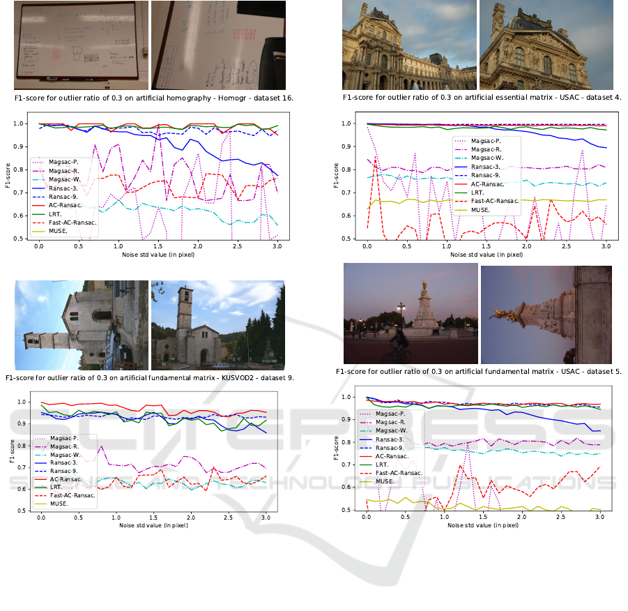
Figure 6: Typical F1-score evolution over inlier noise for a low outlier ratio (0.3). Estimation problem, dataset name and image

pair number can be found in each graph’s title. Magsac-P, Magsac-R and Magsac-W correspond to the metrics presented in

Section 3.3.

is sometimes reached but performance remains over-

all better than other algorithms.

5 DISCUSSION

Differences in runtime can be explained by the num-

ber of iterations in each algorithm as much as their

design. Indeed, each algorithm has to compute

models—which is fast—and compute residuals for all

points—slow. LRT’s high and low speeds likely stem

from its early bailout strategy, skipping residuals en-

tirely. This is a beneﬁt in easy settings, where correct

models are plentiful, but hurts complexity in the op-

posite case, where some rare correct models are not

fully evaluated. AC-RanSaC’s high runtime for large

datasets comes from its sorting step, which takes then

as much time as computing residuals. However, this

may be amended by bucket sorting and discretization

of σ as with LRT to remove sorting entirely. This

is what led to the development of Fast-AC-RanSaC

which shows promising results but could be improved

as its performance is usually worst than that of LRT

that was developped directly in this settings.

StarSAC offers poor performance compared to

other methods except RanSaC. Except in some rare

cases, MUSE’s performance is below that of newer

methods. As explained below, in all settings one of

the newest methods will offer better performance.

Though it is usually the slowest method, AC-

RanSaC shows consistently good precision and re-

call. The algorithm does adapt well to change, and

performs far above baseline in difﬁcult cases. It is a

robust but slower algorithm and except in our most

VISAPP 2022 - 17th International Conference on Computer Vision Theory and Applications

730

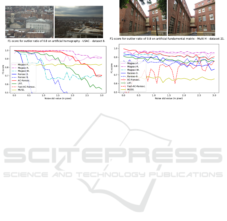
Figure 7: Typical F1-score evolution over inlier noise for a high outlier ratio (0.8). Estimation problem, dataset name and

image pair number can be found in each graph’s title. Magsac-P, Magsac-R and Magsac-W correspond to the metrics presented

in Section 3.3.

complex settings, it produces a good result so it is a

good pick when high classiﬁcation performance is re-

quired.

LRT performed slightly worse than AC-RanSaC,

with selected inlier threshold usually larger, yet much

faster. LRT thus offers a valuable trade-off between

quality and speed. It is however fairly sensitive to the

complexity of the task: a decrease in performance to

baseline level in complex settings and a steep increase

in runtime.

Fast-AC-RanSaC was developped to improve over

AC-RanSaC by reducing runtime but it fails to outper-

form LRT in most cases.

MAGSAC has the potential to perform similarly

or better than AC-RanSaC, at comparable or bet-

ter speeds with impressive performance on the most

complex tasks. It has a very strong resilience to out-

lier and inlier noise and should be used when other al-

gorithms fail to produce a satisfying result. The lack

of robustness of its current implementation makes it

more risky to use ﬁrst hand.

Finally, our semi-artiﬁcial datasets help reveal be-

havior independent of the dataset chosen as initial in-

put, and thus offers new insight in automatic RanSaC

algorithm analysis.

6 CONCLUSION

RanSaC is a robust and efﬁcient algorithm for a wide

range of situations, whose major weaknesses appear

in case of high outlier ratios and unknown inlier noise.

Thanks to a new method to generate semi-synthetic

ground truth data we have made a quantitative evalu-

ation of three major algorithms for noise- and outlier-

robust ﬁtting based on RanSaC. For most standard us-

ages, all algorithms perform well, with only execution

speed varying. When outliers outnumber inliers and

noise is large, adaptive methods justify their existence

by outperforming standard RanSaC by a large mar-

gin, at the cost of speed. Overall, the algorithms offer

a choice for those who seek to trade robustness, ac-

curacy, and execution speed. For example, LRT is a

good algorithm to use on simple cases, offering bet-

ter performance than traditional RanSaC in compara-

ble runtime. MAGSAC has a very strong resilience

to outlier and inlier noise and should be used when

other algorithms fail to produce a satisfying result.

The lack of robustness of its current implementation

makes it more risky to use ﬁrst hand. AC-RanSaC

would then be a more robust but slower algorithm.

Except in our most complex settings, it produces a

good result so it is a good pick when high accuracy

is required. The variety of tests show the strength of

the data generation procedure in exhibiting the sensi-

tivity of the methods to each problem, to noise, and to

outliers.

Thanks to such observations, we plan to im-

prove these methods using the optimizations proposed

above as we did with Fast-AC-RanSaC that proved a

potential improvement if a more stable implementa-

tion can be developped. It is also possible now to per-

form an ablation study of each proposed ingredient

like the σ-consensus post-processing of MAGSAC to

determine precisly their impact on the robustness and

Classiﬁcation Performance of RanSaC Algorithms with Automatic Threshold Estimation

731

retrieval power of each method. Finally, we plan to

extend the study on the remaining model-ﬁtting prob-

lem involved in MVS pipelines: Perspective from n

points (PnP). This problem recovers the camera pose

of a view inserted in the pipeline from 2D-3D cor-

respondences, and model quality measures should be

adapted to that speciﬁc case.

REFERENCES

Barath, D. (2019). MAGSAC implementation. https:

//github.com/danini/magsac. [Online; accessed 22-

January-2021].

Barath, D., Matas, J., and Hajder, L. (2016). Multi-H: Ef-

ﬁcient recovery of tangent planes in stereo images. In

Richard C. Wilson, E. R. H. and Smith, W. A. P., ed-

itors, Proceedings of the British Machine Vision Con-

ference (BMVC), pages 13.1–13.13. BMVA Press.

Barath, D., Matas, J., and Noskova, J. (2019). MAGSAC:

marginalizing sample consensus. In Proceedings of

the IEEE Conference on Computer Vision and Pattern

Recognition (CVPR), pages 10197–10205.

Chin, T.-J., Cai, Z., and Neumann, F. (2018). Robust ﬁtting

in computer vision: Easy or hard? In Proceedings

of the IEEE European Conference of Computer Vision

(ECCV), pages 701–716.

Choi, J. and Medioni, G. (2009). StaRSaC: Stable ran-

dom sample consensus for parameter estimation. In

2009 IEEE Conference on Computer Vision and Pat-

tern Recognition (CVPR), pages 675–682.

Choi, S., Kim, T., and Yu, W. (2009). Performance evalua-

tion of RANSAC family. In Proceedings of the British

Machine Vision Conference (BMVC).

Cohen, A. and Zach, C. (2015). The likelihood-ratio test

and efﬁcient robust estimation. In Proceedings of the

IEEE International Conference on Computer Vision

(ICCV), pages 2282–2290.

Cordts, M., Omran, M., Ramos, S., Rehfeld, T., Enzweiler,

M., Benenson, R., Franke, U., Roth, S., and Schiele,

B. (2016). The cityscapes dataset for semantic urban

scene understanding. In Proc. of the IEEE Conference

on Computer Vision and Pattern Recognition (CVPR).

Dehais, J., Anthimopoulos, M., Shevchik, S., and

Mougiakakou, S. (2017). Two-view 3D reconstruc-

tion for food volume estimation. IEEE Transactions

on Multimedia, 19(5):1090–1099.

Fan, L. and Pylv

ainen, T. (2008). Robust scale estimation

from ensemble inlier sets for random sample consen-

sus methods. In Proceedings of the IEEE European

Conference of Computer Vision (ECCV), pages 182–

195. Springer Berlin Heidelberg.

Fischler, M. and Bolles, R. (1981). Random sample consen-

sus: A paradigm for model ﬁtting with applications to

image analysis and automated cartography. Commu-

nications of the ACM, 24(6):381–395.

Geiger, A., Lenz, P., and Urtasun, R. (2012). Are we ready

for autonomous driving? the kitti vision benchmark

suite. In Conference on Computer Vision and Pattern

Recognition (CVPR).

Hartley, R. and Zisserman, A. (2004). Multiple view geom-

etry in computer vision. Cambridge University Press,

2nd edition. ISBN 978-0521540513.

Isack, H. and Boykov, Y. (2012). Energy-based geomet-

ric multi-model ﬁtting. International Journal of Com-

puter Vision (IJCV), 97(2):123–147.

Leroy, A. M. and Rousseeuw, P. J. (1987). Robust regres-

sion and outlier detection. Wiley series in probability

and mathematical statistics.

Li, Z. and Snavely, N. (2018). MegaDepth: Learning single-

view depth prediction from internet photos. In Pro-

ceedings of the IEEE Conference on Computer Vision

and Pattern Recognition (CVPR), pages 2041–2050.

Lowe, D. G. (2004). Distinctive image features from scale-

invariant keypoints. International Journal of Com-

puter Vision (IJCV), 60(2):91–110.

Magri, L. and Fusiello, A. (2014). T-linkage: A continuous

relaxation of J-linkage for multi-model ﬁtting. In Pro-

ceedings of the IEEE Conference on Computer Vision

and Pattern Recognition (CVPR), pages 3954–3961.

Magri, L. and Fusiello, A. (2015). Robust multiple model

ﬁtting with preference analysis and low-rank approxi-

mation. In Proceedings of the British Machine Vision

Conference (BMVC), pages 20.1–20.12.

Miller, J. V. and Stewart, C. V. (1996). MUSE: Robust sur-

face ﬁtting using unbiased scale estimates. Proceed-

ings of the IEEE Conference on Computer Vision and

Pattern Recognition (CVPR), pages 300–306.

Moisan, L., Moulon, P., and Monasse, P. (2012). Automatic

homographic registration of a pair of images, with a

contrario elimination of outliers. Image Processing

On Line (IPOL), 2:56–73.

Moisan, L., Moulon, P., and Monasse, P. (2016). Funda-

mental matrix of a stereo pair, with a contrario elimi-

nation of outliers. Image Processing On Line (IPOL),

6:89–113.

Moisan, L. and Stival, B. (2004). A probabilistic criterion

to detect rigid point matches between two images and

estimate the fundamental matrix. International Jour-

nal of Computer Vision (IJCV), 57(3):201–218.

Moulon, P. (2012). AC-RanSaC implementation. https:

//github.com/pmoulon/IPOL AC RANSAC. [Online;

accessed 22-January-2021].

Moulon, P., Monasse, P., and Marlet, R. (2012). Adaptive

structure from motion with a contrario model estima-

tion. In Proceedings ot the Asian Conference of Com-

puter Vision (ACCV), pages 257–270. Springer.

Moulon, P., Monasse, P., Perrot, R., and Marlet, R. (2016).

OpenMVG: Open multiple view geometry. In Interna-

tional Workshop on Reproducible Research in Pattern

Recognition, pages 60–74. Springer.

Nist

er, D. (2004). An efﬁcient solution to the ﬁve-

point relative pose problem. IEEE Transactions on

Pattern Analysis and Machine Intelligence (PAMI),

26(6):756–770.

Rabin, J., Delon, J., Gousseau, Y., and Moisan, L. (2010).

MAC-RANSAC: a robust algorithm for the recogni-

tion of multiple objects. Proceedings of the Fifth In-

VISAPP 2022 - 17th International Conference on Computer Vision Theory and Applications

732

ternational Symposium on 3D Data Processing, Visu-

alization and Transmission (3DPVT), pages 51–58.

Raguram, R., Chum, O., Pollefeys, M., Matas, J., and

Frahm, J.-M. (2012). USAC: a universal framework

for random sample consensus. IEEE Transactions

on Pattern Analysis and Machine Intelligence (PAMI),

35(8):2022–2038.

Schonberger, J. L. and Frahm, J.-M. (2016). Structure-

from-motion revisited. In Proceedings of the IEEE

Conference on Computer Vision and Pattern Recogni-

tion (CVPR), pages 4104–4113.

Shotton, J., Glocker, B., Zach, C., Izadi, S., Criminisi, A.,

and Fitzgibbon, A. (2013). Scene coordinate regres-

sion forests for camera relocalization in rgb-d images.

In Proceedings of the IEEE Conference on Computer

Vision and Pattern Recognition, pages 2930–2937.

Toldo, R. and Fusiello, A. (2013). Image-consistent patches

from unstructured points with J-linkage. Image and

Vision Computing, 31:756–770.

Wang, H. and Suter, D. (2004). Robust adaptive-scale para-

metric model estimation for computer vision. IEEE

Transactions on Pattern Analysis and Machine Intel-

ligence (PAMI), 26(11):1459–1474.

Classiﬁcation Performance of RanSaC Algorithms with Automatic Threshold Estimation

733