BRDF-based Irradiance Image Estimation to Remove Radiometric

Differences for Stereo Matching

Kebin Peng

, John Quarles

and Kevin Desai

Department of Computer Science, The University of Texas at San Antonio, Texas, U.S.A.

Keywords:

Bidirectional Reﬂectance Distribution Function, Irradiance, Radiometric Differences, Stereo Matching.

Abstract:

Existing stereo matching methods assume that the corresponding pixels between left and right views have

similar intensity. However, in real situations, image intensity tends to be dissimilar because of the radiometric

differences obtained due to change in light reﬂected. In this paper, we propose a novel approach for removing

these radiometric differences to perform stereo matching effectively. The approach estimates irradiance images

based on the Bidirectional Reﬂectance Distribution Function (BRDF) which describes the ratio of radiance to

irradiance for a given image. We demonstrate that to compute an irradiance image we only need to estimate

the light source direction and the object’s roughness. We consider an approximation that the dot product of the

unknown light direction parameters follows a Gaussian distribution and we use that to estimate the light source

direction. The object’s roughness is estimated by calculating the pixel intensity variance using a local window

strategy. By applying the above steps independently on the original stereo images, we obtain the illumination

invariant irradiance images that can be used as input to stereo matching methods. Experiments conducted on

well-known stereo estimation datasets demonstrate that our proposed approach signiﬁcantly reduces the error

rate of stereo matching methods.

1 INTRODUCTION

Estimating depth from stereo image pairs is one

of the most fundamental tasks in computer vision

(Scharstein and Szeliski, 2002). This task is vital for

many applications, such as 3D reconstruction (Geiger

et al., 2011), robot navigation and control (Song et al.,

2013), object detection and recognition (Chen et al.,

2015). The standard approach is to ﬁnd accurate pixel

correspondence and recover the depth using epipolar

geometry. Approaches for pixel correspondence work

with a color consistency assumption that the pixels in

the left and right views have similar color intensity

values. However, in real situations, the color intensity

values for a given pixel differs between the left and

right views. These differences are known as radiomet-

ric differences. According to (Heo et al., 2010), light

reﬂection and camera setting changes are two main

reasons for having radiometric differences. Light re-

ﬂection is determined by the angle between the direc-

tion of incident ray and the direction of the surface

normal (Heo et al., 2010). The same object surface

https://orcid.org/0000-0003-4866-786X

https://orcid.org/0000-0002-4790-167X

https://orcid.org/0000-0002-2964-8981

could show a different color intensity value if this an-

gle is different. Another typical situation is the differ-

ence in the intensity of the light source. Apart from

light reﬂection, camera settings such as exposure vari-

ations decide the amount of light which reaches the

camera and hence can also cause differences in the

pixel color intensity (Heo et al., 2010).

1.1 Proposed Approach

In this paper, we consider the radiometric differences

in stereo images from the viewpoint of the Bidi-

rectional Reﬂectance Distribution Function (BRDF)

(Walter et al., 2007a). Commonly used in Computer

Graphics, BRDF considers the micro-structure and

light reﬂection features of an object’s surface and de-

scribes the ratio of radiance to irradiance for a given

image. We propose a novel BRDF-based irradiance

image estimation technique for removing radiomet-

ric differences. Different from previous approaches

(Tan and Triggs, 2010; Han et al., 2013) for radio-

metric difference removal that focus on radiance, i.e.

reﬂected light from the object’s surface, we consider

irradiance, i.e. incident light on the object’s surface.

Using mathematical foundations around BRDF,

734

Peng, K., Quarles, J. and Desai, K.

BRDF-based Irradiance Image Estimation to Remove Radiometric Differences for Stereo Matching.

DOI: 10.5220/0010879800003124

In Proceedings of the 17th International Joint Conference on Computer Vision, Imaging and Computer Graphics Theory and Applications (VISIGRAPP 2022) - Volume 5: VISAPP, pages

734-744

ISBN: 978-989-758-555-5; ISSN: 2184-4321

(a) Left image (b) Irradiance image of (a)

Figure 1: ArtL example from Middlebury-14 dataset

(Scharstein and Szeliski, 2002) where left (a) and right (b)

stereo images have different light conditions. (b) and (d) are

the illumination invariant irradiance images corresponding

to (a) and (c), that are computed using our radiometric dif-

ference removal approach.

we demonstrate that to compute an irradiance image

we only need to estimate two parameters - light source

direction and object roughness. In our algorithm, we

do not need to estimate the unknown light direction

parameters separately. Rather only the dot products

for these unit direction vectors need to be estimated,

for which we employ an approximation strategy based

on a Gaussian distribution (see section 3.3). To esti-

mate the surface roughness for the objects in the im-

age, we use a local window approach and estimate the

pixel intensity variance (see section 3.4). As the irra-

diance image is decided by light source intensity and

the distance between light sources and objects, it will

not be affected by light reﬂection, viewing angle and

camera setting changes (see Figures 6(b) and 1(d)).

By using the irradiance image as the input for stereo

matching instead of original stereo image pairs, sig-

niﬁcant performance improvement is obtained for the

state-of-the-art stereo matching methods.

1.2 Contributions

In this paper we make the following contributions:

• A Computer Graphics perspective is provided for

removing the radiometric differences in stereo im-

ages by modeling it with the Bidirectional Re-

ﬂectance Distribution Function (BRDF).

• Irradiance image estimation is proposed for ra-

diometric difference removal, which is robust to

lighting conditions and camera exposure.

• The light source direction is approximated using a

Gaussian distribution and object roughness is es-

timated using local window-based pixel intensity

variance.

• Existing stereo matching methods are signiﬁ-

cantly improved by the use of the estimated irra-

diance images as opposed to the original left and

right stereo images.

2 RELATED WORK

Research in radiometric difference removal can be

broadly classiﬁed into the following three categories:

2.1 Matching Cost Function

Methods in this category aim at performing stereo

matching by proposing matching costs that are robust

on images with radiometric differences. Window-

based mutual information methods (Egnal, 2000;

Fookes et al., 2002; Sarkar and Bansal, 2007) do

not require relative ordering and also have similar ef-

fectiveness in removing the radiometric differences.

Another effective way is to perform segment-wise

stereo matching (Zitnick et al., 2004). (Kim et al.,

2003) uses mutual information with iterative global

graph-cuts to compute matching cost. The hierarchi-

cal calculation of pixel-based matching costs, as pro-

posed in (Hirschmuller, 2007), shows the same ac-

curacy results as compared to the window-based ap-

proach (Kim et al., 2003). Even though these methods

work well in removing radiometric differences, they

require a large local-window size to obtain good per-

formance, which results in a high time consumption.

2.2 Pixel Transformation

Pixel transformation methods use a function to remap

the pixel intensity in an image, making the pixel in-

tensity values obey a speciﬁc distribution or a curve.

(Khan et al., 2015) uses normalized histogram to

make the pixel intensity values obey a uniform distri-

bution. (Deng, 2016; Changyong et al., 2014) apply

log functions on an image to make the pixel inten-

sity values obey a log curve. (Rahman et al., 2016;

Deng, 2016) make the pixel intensity values obey a

gamma curve by applying gamma correction tech-

niques. These pixel-transformation methods work

well only when the background and foreground have

similar pixel intensity. Many techniques have been

proposed to overcome this drawback. (Zhuang and

Guan, 2017) divides the whole image into sub-images

and then normalizes each sub-image by its mean and

BRDF-based Irradiance Image Estimation to Remove Radiometric Differences for Stereo Matching

735

variance-based histogram. (Campos et al., 2019) pro-

poses a machine-learning based approach for hyper-

parameter selection in order to perform a contrast lim-

ited adaptive histogram equalization. However, be-

cause methods in this category only consider the pixel

intensity and ignore the light condition and object ma-

terial, they have not been able to effectively deal with

radiometric differences. Also, because uniform distri-

bution makes pixel intensity similar, histogram meth-

ods, such as (Khan et al., 2015), are more likely to

create blurry disparity maps.

2.3 Reﬂectance Estimation

Methods in this category take a more direct approach

and estimate the reﬂectance from a 2D image, which

is light invariant when objects have the same reﬂec-

tivity. Usually, this idea depends on an illumination

model, e.g., reﬂectance-illumination model. (Xie and

Lam, 2006) proposes a local normalization method

by assuming that objects, faces in their case, consist

of a combination of small facets and remove the ra-

diometric differences by performing normalization on

these facets. (Tan and Triggs, 2010) proposes local

ternary patterns to remove the radiometric differences

by using thresholds for neighboring pixels based on

the value of the central pixel. While the above two

methods estimate reﬂectance indirectly, (Chen et al.,

2006) develops total variation models which consider

a 2D image as the product of light source intensity and

a kernel function. However, selecting a speciﬁc kernel

function may not be applicable to images with varying

light conditions. Moreover, these methods do not con-

sider the object’s micro surface structure which could

inﬂuence the reﬂectance.

In this paper, we exploit the advantages of all the

above three categories to design a radiometric dif-

ference removal algorithm that considers image re-

ﬂectance for all pixels in a given window. As op-

posed to matching cost methods, our approach per-

forms a lot faster as it only considers a static-sized

window. Compared with existing pixel transforma-

tion approaches, our reﬂectance-based method works

on each pixel separately and hence does not result in

a blurry disparity map. Our method performs consis-

tently well on images from a variety of well-known

stereo matching datasets. Our radiometric difference

removal approach is described in Section 3, with the

experiments and results reported in Section 4. We fur-

ther analyze and discuss some of our results in Section

4.7 and provide concluding remarks in Section 5.

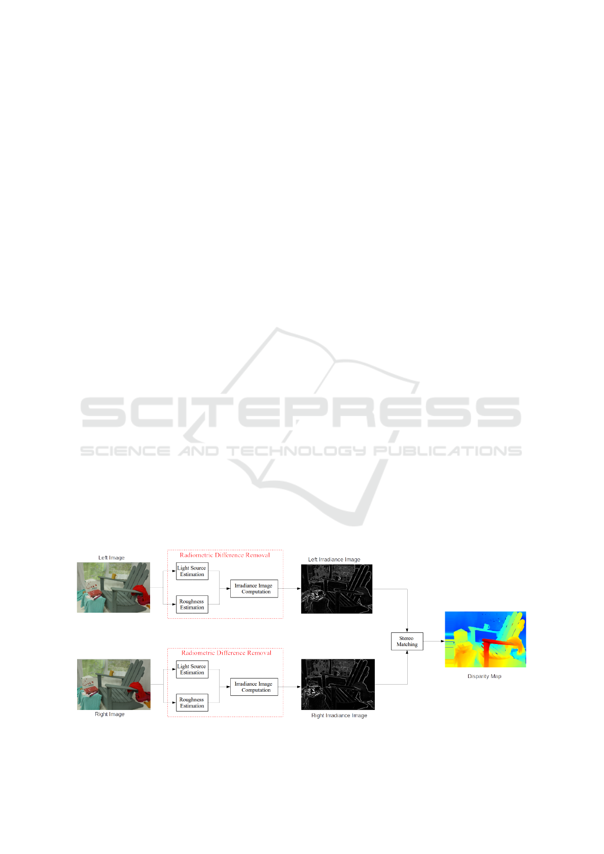
3 PROPOSED APPROACH

The overall objective of our approach is to estimate

the left and right irradiance images by removing the

radiometric differences from the stereo image pairs.

Stereo matching is applied on these irradiance im-

ages instead of the original stereo images to obtain

improved disparity map results. As shown in Fig-

ure 2, the proposed radiometric difference removal

algorithm consists of three parts: (1) irradiance im-

age computation, (2) light direction estimation, and

(3) object roughness estimation.

3.1 Assumptions

A given pixel can receive light from two types of

sources - direct light and indirect light. To simplify

our model, we assume that there is a single direct

light source following other BRDF estimation pa-

pers, e.g., (Chung et al., 2006) and we call it single

light source assumption. Indirect light refers to the

reﬂected light between objects (ambient light). We

Figure 2: Overview of the proposed radiometric difference removal approach for Stereo Matching.

VISAPP 2022 - 17th International Conference on Computer Vision Theory and Applications

736

further assume that ambient light comes from all di-

rections except light source direction with nearly the

same lighting brightness and we call it uniform am-

bient light assumption. With such assumptions, we

use order-0 Spherical Harmonics to model the ambi-

ent light (Sloan et al., 2005).

3.2 Irradiance Image Computation

BRDF, denoted by f

(i, o), is the ratio of scattered ra-

diance L(i) in the direction i to irradiance E(o) from

the direction o. Based on this deﬁnition, we perform

irradiance image estimation using the equation:

E(o) =

L(i)

(i, o)

(1)

Using Microfacet theory, (Walter et al., 2007b)

shows that a roughness term α can be incorporated

into BRDF for describing an object’s micro-surface.

By applying that formulation to our Equation 1, we

obtain the following:

E(o) =

i∈Ω

L(i)4 |i ·n||o · n|

schlick

, h, i)G(n, o, α)D(h)

(2)

The integral in the above equation represents all

possible incoming light for the pixel in the upper

hemisphere (Ω in Equation 3). i is the direction of the

reﬂected light from an object’s surface. o is the direc-

tion of light coming from the light source. n refers to

the direction of the object surface’s normal. h is the

normalized half-vector of i and o. F(i, h) is a Fres-

nel term which describes the reﬂection and transmis-

sion of light when incident on an interface between

different optical media. It is usually approximated us-

ing Fresnel-Schlick function F

schlick

, h, i) (Schlick,

1994) where F

is the reﬂection coefﬁcient for light

incoming parallel to the normal. G(i, o, α) is the Ge-

ometrical Attenuation Factor (Kelemen and Szirmay-

Kalos, 2001) which describes what percentage of the

reﬂected light will not be blocked by the surface to-

pography (Hao et al., 2019). D(h) is the GGX Distri-

bution Function (Walter et al., 2007a) which describes

the probability distribution of the surface normal.

To solve Equation 3, we ﬁrst discuss the possi-

ble incoming light directions in the upper hemisphere

for a pixel. According to single light source assump-

tion in Section 3.1, the direct light only has one di-

rection, which is the light source direction. However,

the indirect light has unlimited directions in the upper

hemisphere. Here, we apply uniform ambient light

assumption, as mentioned in Section 3.1. That is,

the ambient light comes in all directions except light

source direction with nearly the same lighting bright-

ness. So the ambient can be viewed as a constant C.

Intuitively, We may set C as the mean value of input

images, or we could use 0-order Spherical Harmonics

function (Sloan et al., 2005), which is

4π

, to model

the ambient light. So Equation 3 can be simpliﬁed as:

E(o) =

L(i)4 |i ·n||o · n|

schlick

, h, i)G(n, o, α)D(h)

+C (3)

Next, we estimate the reﬂected light L(i) as received

by the camera by mapping it to image pixel inten-

sity. This is modeled by the camera response function

which, according to (Ng et al., 2007), is assumed to

be a gamma curve that is generally approximated by

a polynomial function. We compared different types

of polynomial approximations (linear, quadratic, etc.)

and found no signiﬁcant difference between them.

Hence, in our approach we approximate the camera

response function using a linear function which im-

plies that L(i) is the same as image intensity.

After solving for L(i), the only unknown variables

that need to be estimated are i, o, n, h, and α. The

ﬁrst four parameters are associated with the light di-

rection, whereas the last parameter is the object sur-

face roughness. Considering theoretical foundations

and expansion of the functions in Equation 3, param-

eters i, o, n, and h are never used on their own. Rather,

they are always used in combinations as a dot product.

In Section 3.3, we demonstrate that the dot product

of any of these parameters obeys a Gaussian distribu-

tion, based on which we estimate the light direction.

We estimate the surface roughness α using a local

window-based approach for pixel intensity variance,

shown in Section 3.4.

3.3 Light Direction Estimation

As mentioned above, light source direction can be es-

timated by approximating the dot products of i, o, n,

and h. We demonstrate that any combination of the

dot products of these direction vectors follow a Gaus-

sian distribution.

Assume a and b are any of the four direction vec-

tors i, o, n, and h. The dot product of a and b can

be represented as a · b =

cosθ. These vectors

are normalized unit direction vectors. Hence, the dot

product is dependent on just the cosine of the angle θ

between a and b i.e. cos θ. As we do not know the

angle between these vectors, we cannot ﬁnd the value

for cos θ. Considering that θ ∈ [−π, π], by selecting

speciﬁc values for µ and σ

, we can plot the function

graph for the Gaussian distribution N(µ, σ

). Visual

comparison shows that this Gaussian function graph

is very similar to the function graph for cos θ. Hence,

BRDF-based Irradiance Image Estimation to Remove Radiometric Differences for Stereo Matching

737

we use Gaussian distribution to approximate the value

for cosθ.

In Equation 3, we estimate the irradiance value for

each pixel of an image of length l and height h. We

need to obtain a speciﬁc dot product value for the four

direction vectors i, o, n, and h. Hence, we generate

a Gaussian distribution N(µ, σ

) for l ∗ h values and

pick the value that matches the row and column value

for the corresponding image. This value is used for

the light source direction estimation.

3.4 Roughness Estimation

As mentioned in Section 3.2, we need to estimate

the object surface roughness α in order to compute

the irradiance images. Surface element roughness de-

scribes how ﬂat (low roughness) or how rugged (high

roughness) a surface is at a micro level. It is depen-

dent on the object’s material and is usually set manu-

ally according to a visual understanding of the object

in the image. However, in stereo image pairs consist-

ing of multiple objects, it is not possible to effectively

set an appropriate value manually.

According to BRDF (Walter et al., 2007a), sur-

face roughness has an inverse relationship with local

pixel intensity variance. If the object surface has high

roughness, the reﬂected light would be more likely to

be scattered into different directions. This difference

in light direction could make the image seem blurry

indicating that it has smaller pixel intensity variance.

We design a local window-based approach to approx-

imate the pixel intensity variance which leads to the

estimation of surface roughness α based on the fol-

lowing equation:

α =

(p)

∑

i=1

∑

j=1

i j

− M

(p))

(4)

where p is the center pixel for which we are trying

to estimate the pixel intensity variance V

(p) in a lo-

cal square window of size t (an odd number). M

(p)

denotes the mean pixel intensity value in this window.

Based on the approach mentioned above in Sec-

tions 3.2, 3.3, and 3.4, we compute the left and right

irradiance images for the original stereo image pairs.

The radiometric differences are removed in these irra-

diance images which can then be applied to any stereo

matching method.

4 EXPERIMENTS

In this section, we conduct extensive experimental

analysis to evaluate the effectiveness of our radiomet-

ric difference removal algorithm on stereo matching.

Left Image

SGBM2

ELAS

PSMNet

OVOD

SGBM2*

ELAS*

OVOD*

PSMNet*

LocalExp

HSM-Net

AANet++

CRL

RAFT-Stereo

LEAStereo

LocalExp*

HSM-Net*

AANet++*

CRL*

RAFT-Stereo*

LEAStereo*

Right Image

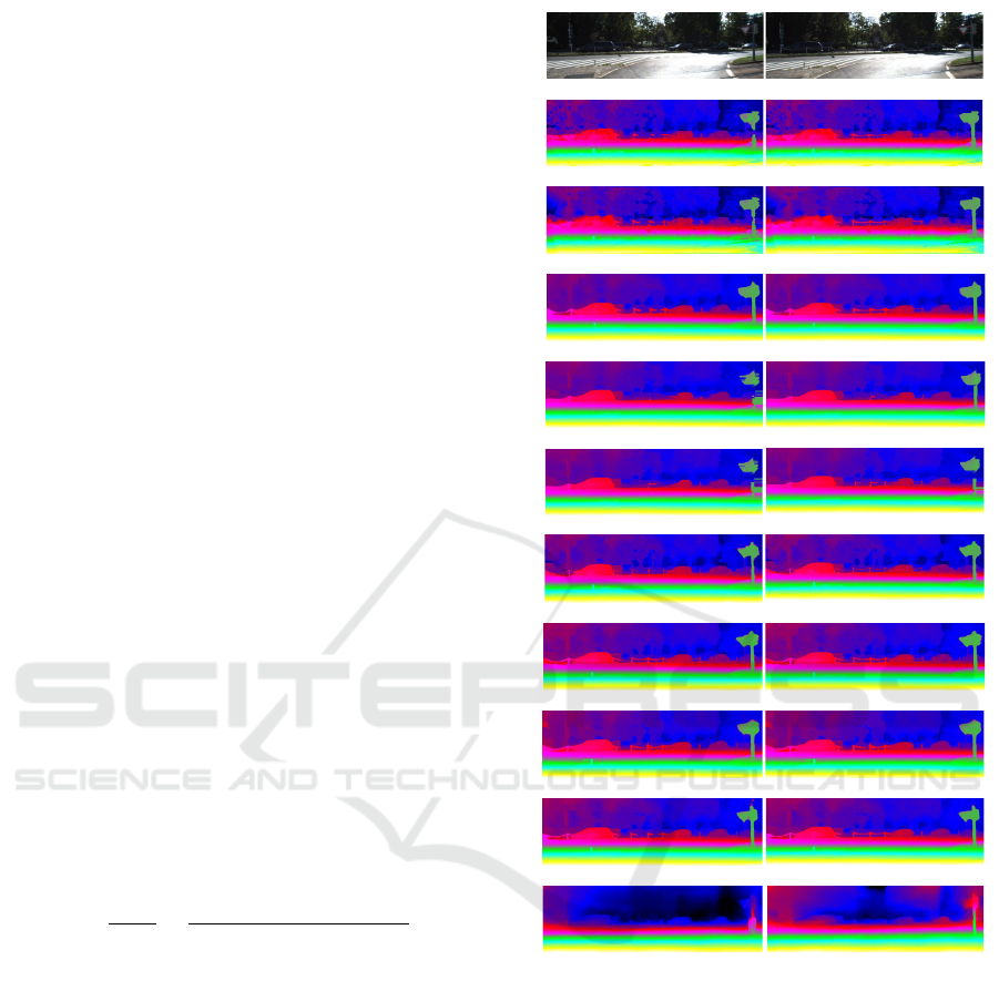
Figure 3: An example image from the test set (so no ground

truth) of KITTI-15 dataset (Scharstein et al., 2014).

de-

notes the use of our approach prior to applying the stereo

matching methods.

4.1 Implementation Details

All the experiments are conducted on a computer hav-

ing a 2.6 GHz CPU with an i7 processor and 32 GB

RAM. Our radiometric removal algorithm for con-

verting the original stereo images to irradiance im-

ages is implemented in C++. For the Fresnel-Schlick

function (Schlick, 1994) used in Equation 3, we use

linear base reﬂectivity and set F

= 0.365. We con-

ducted a separate experiment and found that there

were no major differences in our results across dif-

ferent F

values. We picked the value which gave

VISAPP 2022 - 17th International Conference on Computer Vision Theory and Applications

738

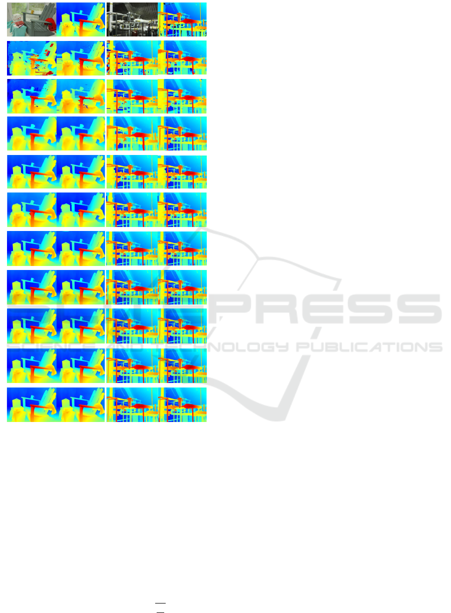
Adirondack

SGBM2

ELAS

PSMNet

OVOD

LocalExp

HSM-Net

AANet++

CRL

RAFT-Stereo

LEAStereo

Ground Truth

SGBM2*

ELAS*

PSMNet

OVOD*

LocalExp*

HSM-Net*

AANet++*

CRL*

RAFT-Stereo*

LEAStereo*

Pipes

SGBM2

ELAS

PSMNet

OVOD

LocalExp

HSM-Net

AANet++

CRL

RAFT-Stereo

LEAStereo

Ground Truth

SGBM2*

ELAS*

PSMNet*

OVOD*

LocalExp*

HSM-Net*

AANet++*

CRL*

RAFT-Stereo*

LEAStereo*

Figure 4: Adirondack image and Pipes image from the

Middlebury-14 dataset (Scharstein et al., 2014) along with

the ground truth disparity map. First and third columns

show the disparity maps generated by 10 stereo matching

methods on the original stereo image pairs. Second and

fourth columns show results on the irradiance images esti-

mated by our radiometric difference removal algorithm (de-

noted by

the best results. We did the same for the Gaussian

distribution N(µ, σ

) parameters and set them to be

µ = 10 and σ = 1. The Gaussian distribution is then

used as an approximation of cos θ in estimating the

light direction (see Section 3.3). In Equation 4 we se-

lect the local square window size to be t = 5 because

we ﬁnd that it results in the best performance. Also,

we set ambient light constant C =

4π

as it yields

better results. Implementation details of the different

stereo matching methods we use in our experiments

are mentioned in Section 4.3.

4.2 Datasets & Evaluation Metrics

We use three popular stereo matching datasets and the

corresponding evaluation metrics.

• Middlebury-14 (Scharstein et al., 2014) is a high-

resolution two-view dataset that consist of multi-

ple stereo images of indoor scenes. We use the 15

training stereo image pairs and focus only on the

non-occluded pixels during evaluation. avgerr,

bad-0.5, bad-1.0, and bad-2.0 are used as the eval-

uation metrics for this dataset.

• Middlebury-06 (Hirschmuller and Scharstein,

2007) is the older version of the Middlebury-

14 dataset. We use this to evaluate our method

against other pre-processing methods in differ-

ent lighting and exposure conditions. We use the

avgerr metric to graph the comparisons.

• KITTI-15 (Menze et al., 2018) dataset is also

used to evaluate the impact of our proposed

pre-processing method on other stereo matching

methods. We perform analysis on all the 200 low

resolution stereo pairs. The metrics used for this

dataset are D1-all, D1-bg and D1-fg, which refer

to the percentage of outliers for all pixels, back-

ground pixels, and foreground pixels respectively.

For all experiments, we use

to denote the use of our

radiometric removal algorithm with the correspond-

ing stereo matching method or evaluation metric.

4.3 Stereo Matching Estimation

Methods Compared

Several pre-processing optimization approaches exist

for improving stereo matching, such as (Heo et al.,

2012) and (Zhou and Boulanger, 2012), which are il-

lumination invariant approaches. However, these ap-

proaches also change the cost function and hence can-

not directly be compared with our approach. Radio-

metric invariant ﬁlters such as gradient, census, and

rank ﬁlters can also be used for optimizing stereo

matching. These ﬁlters also depend on the cost func-

tion. On the other hand, our approach is separate from

the cost function. This is the major advantage of our

method that it can work with any stereo matching al-

gorithms using their individual cost functions.

The irradiance images obtained from our radio-

metric removal algorithm are used as input for 10

representative state-of-the-art stereo matching meth-

ods: SGBM2 (Hirschmuller, 2007), ELAS (Geiger

BRDF-based Irradiance Image Estimation to Remove Radiometric Differences for Stereo Matching

739

et al., 2010), AANet++ (Xu and Zhang, 2020),

PSMNet (Chang and Chen, 2018), HSM-Net (Yang

et al., 2019), LEAStereo (Cheng et al., 2020),Lo-

calExp (Taniai et al., 2017), OVOD (Mozerov and

van de Weijer, 2019),CRL (Pang et al., 2017), RAFT-

Stereo (Lipson et al., 2021). For Figure 4 shows the

disparity maps for the Adirondack image and Pipes

image in the Middlebury-14 dataset. For all meth-

ods, except SGBM2, we directly use implementations

available online on their respective GitHub reposito-

ries. However, we do need to ﬁne-tune speciﬁc pa-

rameters in their models to obtain the reported re-

sults on different datasets. We implement SGBM2

(Hirschmuller, 2007) using OpenCV by setting the

following parameter values to accurately replicate re-

sults: SAD window size = 3, truncation value for pre-

ﬁlter = 63, P1 = 8 ∗ 3 ∗ 3, P2 = 32 ∗ 3 ∗ 3, uniqueness

ratio = 10, speckle window size = 100, speckle range

= 32, max disparity value = 128. We also set the in-

put image resolution to be half of the original.

Here, we perform experimental analysis on each

of the four datasets and report the results for the same.

Middlebury-14 Dataset (Scharstein et al., 2014):

Figure 4 shows visual disparity map results for the

Adirondack image from the Middlebury-14 dataset

(Scharstein et al., 2014). As visible in the dispar-

ity maps, the results obtained on the stereo matching

methods after applying our radiometric removal algo-

rithm (bottom row) are better compared to the ones

obtained without using our algorithm (top row). The

dataset consists of 15 stereo image pair test cases on

which we conduct our analysis. We conduct exper-

iments for all 10 stereo matching methods on these

image pairs using avgerr, bad-0.5, bad-1.0, and bad-

2.0 as the evaluation metrics.

Table 1 shows the results for our experimental

analysis. In the majority of the cases, we obtain a re-

duction in the error rates indicating the effectiveness

of our algorithm for stereo matching. For example,

we obtain avgerr reduction of 34.43% for SGBM2

and 6.12% for AANet++. The worst performance is

for HSM-Net where avgerr increases by 1.41%.

KITTI-15 Dataset (Menze et al., 2018): We report

results for all the three percentages of outliers metrics

that are generally used for this dataset - D1-all, D1-

bg, and D1-fg. Table 2 shows the results for all the

10 stereo matching methods with and without the use

of our algorithm. As shown in the table, by using our

algorithm, all methods report performance improve-

ment across all metrics. For example, for D1-all, error

reduction is obtained in the range of 1.05%−37.99%.

Figure 3 shows visual disparity map results for an ex-

ample image from the test set in KITTI-15 Dataset.

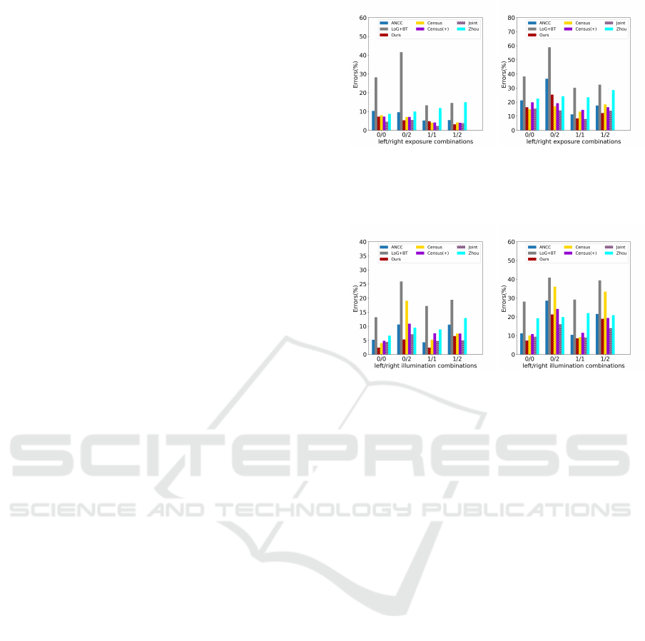
(a) Aloe (b) Art

Figure 5: Comparison of our approach with other pre-

processing approaches for camera exposure changes on

three images from the Middlebury-06 dataset (Hirschmuller

and Scharstein, 2007).

(a) Aloe (b) Art

Figure 6: Comparison of our approach with other pre-

processing approaches for changes in the light source on

three images from the Middlebury-06 dataset (Hirschmuller

and Scharstein, 2007).

4.4 Robustness to Camera Exposure &

Light Source Changes

We also evaluate the robustness of our approach

across different camera exposure settings as well as

changes to the light source. We use two different im-

ages from the Middlebury-06 dataset (Hirschmuller

and Scharstein, 2007) to compare our approach with

the ﬁve other pre-processing approaches. For this

analysis, we use the same experimental setting as in

the ANCC work (Heo et al., 2008). Also, same as in

(Heo et al., 2012), we have included Census(+) in our

evaluation which uses a combined log-chromaticity

color (70% weight) and RGB color (30% weight).

Figure 5 shows the two comparison graphs with

each having four different camera exposure combina-

tions between the left and the right views. Similarly,

Figure 6 shows the comparison graphs for light source

changes. As seen from the graphs, our approach out-

performs most other pre-processing approaches in all

the four combinations for left/right views, for both

camera exposure and light source changes.

VISAPP 2022 - 17th International Conference on Computer Vision Theory and Applications

740

Table 1: Results on the Middlebury-14 (Scharstein et al., 2014) training set for 10 stereo matching methods (our algorithm

denoted by

). Percentage change in the error values is shown in parenthesis with an arrow indicating increase or decrease.

Method Res avgerr avgerr

bad-0.5 bad-0.5

bad-1.0 bad-1.0

bad-2.0 bad-2.0

SGBM2 F 11.15 7.31 (34.43%↓) 56.71 38.60 (31.93%↓) 36.18 24.43 (32.4%↓) 27.52 23.57 (14.35%↓)

ELAS F 7.56 7.62 (0.79%↑) 61.62 60.58 (1.68%↓) 38.73 37.27 (0.65%↓) 27.88 26.18 (0.93%↓)

PSMNet Q 9.92 9.87 (0.50%↓) 89.98 98.90 (9.91%↑) 78.34 77.83 (3.76%↓) 59.11 58.56 (6.09%↓)

OVOD H 1.82 1.79 (1.64%↓) 38.22 37.81 (1.07%↓) 17.91 17.75 (0.89%↓) 9.67 9.53 (1.44%↓)

LocalExp H 1.76 1.74 (1.13%↓) 38.45 38.17 (0.72%↓) 14.32 14.20 (0.83%↓) 6.43 6.31 (1.86%↓)

HSM-Net F 1.41 1.43 (1.41%↑) 50.29 49.61 (1.35%↓) 22.99 23.24 (1.08%↑) 10.78 10.83 (0.46% ↑)

CRL H 1.45 1.43(1.38%↓) 47.35 46.18(2.47%↓) 19.53 19.19(1.74%↓) 12.71 12.54(1.33%↓)

RAFT-Stereo H 1.04 0.98(5.76%↓) 28.61 25.42(11.1%↓) 10.60 10.12(4.52%↓) 5.25 4.92(6.28%↓)

LEAStereo H 1.09 1.03 (5.5%↓) 36.10 35.71 (1.08%↓) 18.40 17.91 (2.7%↓) 2.47 2.52 (2.02% ↑)

AANet++ H 0.98 0.92 (6.12%↓) 33.18 31.95 (3.70%↓) 12.18 11.49 (5.66%↓) 5.65 5.09 (9.91%↓)

Table 2: Results on the KITTI-15 dataset (Menze et al., 2018) with D1-all, D1-bg, and D1-fg evaluation metrics. Superscript

(e.g., D1-all

) denotes the use of our algorithm prior to applying the stereo matching methods. Percentage change in the error

values is shown in parenthesis with an arrow indicating increase or decrease.

Method D1-all D1-all

D1-bg D1-bg

D1-fg D1-fg

SGBM2 6.87 4.26 (37.99%↓) 15.29 11.68 (23.61%↓) 5.15 4.27 (17.08%↓)

ELAS 9.78 8.14 (16.85%↓) 19.04 14.93 (21.58%↓) 7.86 5.42 (31.04%↓)

PSMNet 2.32 2.24 (3.44%↓) 1.88 1.64 (12.36%↓) 4.65 4.39 (5.59%↓)

OVOD 4.21 3.9 (7.36%↓) 3.21 3.23 (0.62%↑) 5.94 5.28 (11.11%↓)

LocalExp 4.76 4.71 (1.05%↓) 3.52 3.78 (7.38%↑) 7.47 6.21 (16.86%↓)

HSM-Net 2.19 2.05 (6.39%↓) 1.82 1.76 (3.29%↓) 3.86 3.71 (3.88%↓)

CRL 2.15 2.14(0.46%↓) 2.25 2.21(1.77%↓) 3.41 3.43(0.58%↑)

RAFT-Stereo 1.96 1.73(11.7%↓) 1.75 1.66(5.14%↓) 2.89 2.69 (6.92%↓)

LEAStereo 1.65 1.73 (3.03%↑) 1.40 1.43(2.14 %↑) 2.91 2.93 (0.69%↑)

AANet++ 2.31 2.02 (12.55%↓) 2.10 1.94 (7.61%↓) 5.35 5.22 (2.43%↓)

Table 3: Comparison of our approach with ﬁve other pre-processing approaches when used in conjunction with all the 10

stereo matching methods. We report the average error obtained on the Middlebury-14 dataset (Scharstein et al., 2014). Best

result is marked in bold.

Method

Pre-processing

Ours Census LoG ANCC Joint Zhou

SGBM2 11.5 7.31 7.96 9.15 15.81 12.64 16.72

ELAS 7.56 7.62 13.06 15.54 7.16 7.14 22.58

PSMNet 9.92 9.87 12.24 12.63 8.40 7.28 18.63

OVOD 1.82 1.79 1.93 2.65 1.73 1.75 5.11

LocalExp 1.76 1.74 2.24 3.43 2.28 2.30 9.98

HSM-Net

1.41 1.43 1.39 4.34 2.45 2.43 7.52

CRL 1.45 1.43 1.47 4.69 2.72 2.30 6.85

RAFT-Stereo 1.04 0.98 1.52 1.31 1.49 1.23 1.77

LEAStereo 1.09 1.03 2.02 1.89 3.15 3.37 3.95

AANet++ 0.98 0.92 1.49 4.07 3.65 3.43 4.84

4.5 Comparison with Other

Pre-processing Methods

As ours is a pre-processing method, we also com-

pare it with ﬁve other pre-processing methods that

use radiometric invariant ﬁlters, namely ANCC (Heo

et al., 2008) that uses Chromaticity normalization,

Laplacian of Gaussian (LoG) + BT (Birchﬁeld and

Tomasi, 1998), Census (7 × 7) (Zabih and Woodﬁll,

1994) + Hamming, Joint (Heo et al., 2012) that uses

Log Chromaticity normalization, and Zhou (Zhou and

Boulanger, 2012) that uses Relative Gradients. Be-

cause our approach is separate from the stereo match-

ing algorithm, we use BT (Birchﬁeld and Tomasi,

1998) as our stereo matching algorithm for fair com-

parison. We use GraphCut (GC) to optimize all the

matching costs as the same as (Heo et al., 2012).

In Table 3, we report the avgerr results for ours

and each of the ﬁve other pre-processing approaches

when used in conjunction with the 10 state-of-the-

BRDF-based Irradiance Image Estimation to Remove Radiometric Differences for Stereo Matching

741

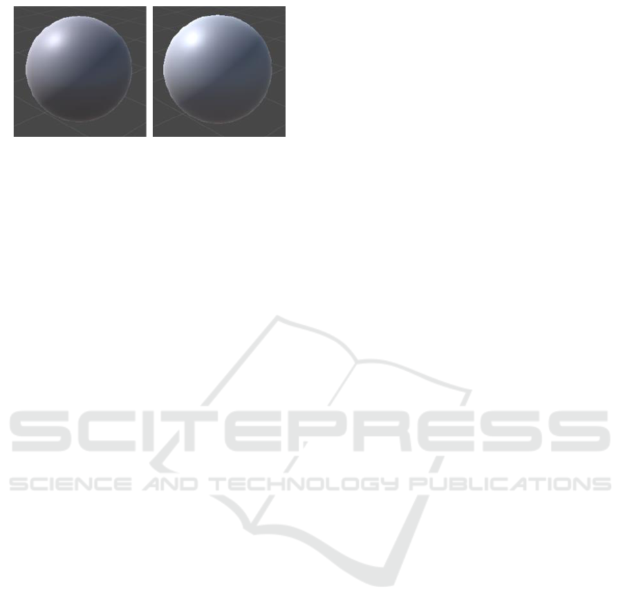
(a) Origianl Sphare (b) Simulated Sphare

Figure 7: Comparison of our original image and our re-

rendered image. (a) is rendered with the original BRDF

model (b) is re-rendered with our estimated BRDF value.

art stereo matching algorithms. As seen from the re-

sults, our approach improves the performance by re-

ducing the errors signiﬁcantly for all 10 stereo match-

ing methods, as opposed to the other pre-processing

approaches that use radiometric invariant ﬁlters.

4.6 Validation of BRDF Estimation

We evaluated the accuracy of BRDF estimation using

a simulated image, as it is difﬁcult to obtain the ac-

tual BRDF ground truth values. We ﬁrst use Unity3

to render the original image (a) with our own BRDF

shader, so the ground-truth BRDF values are known.

Then we use our proposed approach to estimate the

BRDF for image (a). At last, we use this estimated

BRDF to render a new reconstructed image, which

we compare with the original image. Figure 7 shows

the results for two different images where we com-

pare the original (a) and the simulated images (b) to

visually validate the accuracy of the proposed BRDF

estimation approach.

4.7 Limitations & Future Work

Our approach for irradiance image computation esti-

mates the light source direction statistically. So there

is a difference between our estimated value and the

real value for the light source direction. We will

investigate such differences in the future. In gen-

eral Computer Graphics, the lighting function is pre-

known and can be used to estimate the ambient light.

However, in our approach the lighting function is un-

known. Hence, we plan to investigate the estimation

of the ambient light constant C by using Monte Carlo

Sampling Methods in the future.

5 CONCLUSIONS

In this paper we propose a novel radiometric dif-

ference removal algorithm for improving the perfor-

mance of stereo matching methods. The approach is

based on the Computer Graphics concept of BRDF

to compute the irradiance images for the original left

and right stereo images. For doing so, we estimate the

light source direction by considering an approxima-

tion that the dot product of the unknown light direc-

tion parameters follows a Gaussian distribution. We

estimate the object’s roughness by employing a lo-

cal window strategy and calculating the pixel inten-

sity variance. The obtained irradiance images are ro-

bust to changes in illumination, exposure, and light

source intensity. These images when used as input

for stereo matching methods improve the quality of

the generated disparity maps as opposed to the ones

obtained while running the methods on the original

stereo images. Results on the experiments performed

on 10 stereo matching methods show signiﬁcant per-

formance improvement for disparity map generation.

REFERENCES

Birchﬁeld, S. and Tomasi, C. (1998). A pixel dissimilarity

measure that is insensitive to image sampling. IEEE

Transactions on Pattern Analysis and Machine Intel-

ligence, 20(4):401–406.

Campos, G. F. C., Mastelini, S. M., Aguiar, G. J., Manto-

vani, R. G., de Melo, L. F., and Barbon, S. (2019). Ma-

chine learning hyperparameter selection for contrast

limited adaptive histogram equalization. EURASIP

Journal on Image and Video Processing, 2019(1):59.

Chang, J.-R. and Chen, Y.-S. (2018). Pyramid stereo match-

ing network. In Proceedings of the IEEE Conference

on Computer Vision and Pattern Recognition, pages

5410–5418.

Changyong, F., Hongyue, W., Naiji, L., Tian, C., Hua, H.,

Ying, L., et al. (2014). Log-transformation and its im-

plications for data analysis. Shanghai archives of psy-

chiatry, 26(2):105.

Chen, T., Yin, W., Zhou, X. S., Comaniciu, D., and Huang,

T. S. (2006). Total variation models for variable light-

ing face recognition. IEEE transactions on pattern

analysis and machine intelligence, 28(9):1519–1524.

Chen, X., Kundu, K., Zhu, Y., Berneshawi, A. G., Ma, H.,

Fidler, S., and Urtasun, R. (2015). 3d object propos-

als for accurate object class detection. In Advances in

Neural Information Processing Systems, pages 424–

432.

Cheng, X., Zhong, Y., Harandi, M., Dai, Y., Chang, X., Li,

H., Drummond, T., and Ge, Z. (2020). Hierarchical

neural architecture search for deep stereo matching.

Advances in Neural Information Processing Systems,

33.

Chung, A. J., Deligianni, F., Shah, P., Wells, A., and

Yang, G.-Z. (2006). Patient-speciﬁc bronchoscopy vi-

sualization through brdf estimation and disocclusion

correction. IEEE transactions on medical imaging,

25(4):503–513.

VISAPP 2022 - 17th International Conference on Computer Vision Theory and Applications

742

Deng, G. (2016). A generalized gamma correction algo-

rithm based on the slip model. EURASIP Journal on

Advances in Signal Processing, 2016(1):69.

Egnal, G. (2000). Mutual information as a stereo correspon-

dence measure.

Fookes, C., Bennamoun, M., and Lamanna, A. (2002). Im-

proved stereo image matching using mutual informa-

tion and hierarchical prior probabilities. In Object

recognition supported by user interaction for service

robots, volume 2, pages 937–940. IEEE.

Geiger, A., Roser, M., and Urtasun, R. (2010). Efﬁcient

large-scale stereo matching. In Asian conference on

computer vision, pages 25–38. Springer.

Geiger, A., Ziegler, J., and Stiller, C. (2011). Stereoscan:

Dense 3d reconstruction in real-time. In 2011 IEEE

intelligent vehicles symposium (IV), pages 963–968.

Ieee.

Han, H., Shan, S., Chen, X., and Gao, W. (2013). A com-

parative study on illumination preprocessing in face

recognition. Pattern Recognition, 46(6):1691–1699.

Hao, D., Wen, J., Xiao, Q., You, D., and Tang, Y.

(2019). An improved topography-coupled kernel-

driven model for land surface anisotropic reﬂectance.

IEEE Transactions on Geoscience and Remote Sens-

ing.

Heo, Y. S., Lee, K. M., and Lee, S. U. (2008). Illumination

and camera invariant stereo matching. In 2008 IEEE

Conference on Computer Vision and Pattern Recogni-

tion, pages 1–8. IEEE.

Heo, Y. S., Lee, K. M., and Lee, S. U. (2010). Robust stereo

matching using adaptive normalized cross-correlation.

IEEE Transactions on Pattern Analysis and Machine

Intelligence, 33(4):807–822.

Heo, Y. S., Lee, K. M., and Lee, S. U. (2012). Joint depth

map and color consistency estimation for stereo im-

ages with different illuminations and cameras. IEEE

transactions on pattern analysis and machine intelli-

gence, 35(5):1094–1106.

Hirschmuller, H. (2007). Stereo processing by semiglobal

matching and mutual information. IEEE Transac-

tions on pattern analysis and machine intelligence,

30(2):328–341.

Hirschmuller, H. and Scharstein, D. (2007). Evaluation of

cost functions for stereo matching. In 2007 IEEE Con-

ference on Computer Vision and Pattern Recognition,

pages 1–8. IEEE.

Kelemen, C. and Szirmay-Kalos, L. (2001). A microfacet

based coupled specular-matte brdf model with impor-

tance sampling. In Eurographics short presentations,

volume 25, page 34.

Khan, M. F., Khan, E., and Abbasi, Z. (2015). Image con-

trast enhancement using normalized histogram equal-

ization. Optik, 126(24):4868–4875.

Kim, J. et al. (2003). Visual correspondence using energy

minimization and mutual information. In Proceed-

ings Ninth IEEE International Conference on Com-

puter Vision, pages 1033–1040. IEEE.

Lipson, L., Teed, Z., and Deng, J. (2021). Raft-stereo: Mul-

tilevel recurrent ﬁeld transforms for stereo matching.

arXiv preprint arXiv:2109.07547.

Menze, M., Heipke, C., and Geiger, A. (2018). Object scene

ﬂow. ISPRS Journal of Photogrammetry and Remote

Sensing (JPRS).

Mozerov, M. G. and van de Weijer, J. (2019). One-view

occlusion detection for stereo matching with a fully

connected crf model. IEEE Transactions on Image

Processing, 28(6):2936–2947.

Ng, T.-T., Chang, S.-F., and Tsui, M.-P. (2007). Using ge-

ometry invariants for camera response function esti-

mation. In 2007 IEEE Conference on Computer Vision

and Pattern Recognition, pages 1–8. IEEE.

Pang, J., Sun, W., Ren, J. S., Yang, C., and Yan, Q. (2017).

Cascade residual learning: A two-stage convolutional

neural network for stereo matching. In Proceedings of

the IEEE International Conference on Computer Vi-

sion Workshops, pages 887–895.

Rahman, S., Rahman, M. M., Abdullah-Al-Wadud, M., Al-

Quaderi, G. D., and Shoyaib, M. (2016). An adaptive

gamma correction for image enhancement. EURASIP

Journal on Image and Video Processing, 2016(1):1–

13.

Sarkar, I. and Bansal, M. (2007). A wavelet-based multires-

olution approach to solve the stereo correspondence

problem using mutual information. IEEE Transac-

tions on Systems, Man, and Cybernetics, Part B (Cy-

bernetics), 37(4):1009–1014.

Scharstein, D., Hirschm

uller, H., Kitajima, Y., Krathwohl,

G., Ne

c, N., Wang, X., and Westling, P. (2014).

High-resolution stereo datasets with subpixel-accurate

ground truth. In German conference on pattern recog-

nition, pages 31–42. Springer.

Scharstein, D. and Szeliski, R. (2002). A taxonomy and

evaluation of dense two-frame stereo correspondence

algorithms. International journal of computer vision,

47(1-3):7–42.

Schlick, C. (1994). An inexpensive brdf model for

physically-based rendering. In Computer graphics fo-

rum, volume 13, pages 233–246. Wiley Online Li-

brary.

Sloan, P.-P., Luna, B., and Snyder, J. (2005). Local, de-

formable precomputed radiance transfer. ACM Trans-

actions on Graphics (TOG), 24(3):1216–1224.

Song, D.-l., Jiang, Q.-l., Sun, W.-c., et al. (2013). A sur-

vey: Stereo based navigation for mobile binocular

robots. In Robot Intelligence Technology and Appli-

cations 2012, pages 1035–1046. Springer.

Tan, X. and Triggs, B. (2010). Enhanced local texture fea-

ture sets for face recognition under difﬁcult lighting

conditions. IEEE transactions on image processing,

19(6):1635–1650.

Taniai, T., Matsushita, Y., Sato, Y., and Naemura, T. (2017).

Continuous 3d label stereo matching using local ex-

pansion moves. IEEE transactions on pattern analysis

and machine intelligence, 40(11):2725–2739.

Walter, B., Marschner, S. R., Li, H., and Torrance, K. E.

(2007a). Microfacet models for refraction through

rough surfaces. In Proceedings of the 18th Eurograph-

ics Conference on Rendering Techniques, EGSR’07,

page 195–206, Goslar, DEU. Eurographics Associa-

tion.

BRDF-based Irradiance Image Estimation to Remove Radiometric Differences for Stereo Matching

743

Walter, B., Marschner, S. R., Li, H., and Torrance, K. E.

(2007b). Microfacet models for refraction through

rough surfaces. Rendering techniques, 2007:18th.

Xie, X. and Lam, K.-M. (2006). An efﬁcient illumination

normalization method for face recognition. Pattern

Recognition Letters, 27(6):609–617.

Xu, H. and Zhang, J. (2020). Aanet: Adaptive aggregation

network for efﬁcient stereo matching. In Proceedings

of the IEEE/CVF Conference on Computer Vision and

Pattern Recognition, pages 1959–1968.

Yang, G., Manela, J., Happold, M., and Ramanan, D.

(2019). Hierarchical deep stereo matching on high-

resolution images. In Proceedings of the IEEE Con-

ference on Computer Vision and Pattern Recognition,

pages 5515–5524.

Zabih, R. and Woodﬁll, J. (1994). Non-parametric local

transforms for computing visual correspondence. In

European conference on computer vision, pages 151–

158. Springer.

Zhou, X. and Boulanger, P. (2012). Radiometric invari-

ant stereo matching based on relative gradients. In

2012 19th IEEE International Conference on Image

Processing, pages 2989–2992. IEEE.

Zhuang, L. and Guan, Y. (2017). Image enhancement

via subimage histogram equalization based on mean

and variance. Computational intelligence and neuro-

science, 2017.

Zitnick, C. L., Kang, S. B., Uyttendaele, M., Winder, S.,

and Szeliski, R. (2004). High-quality video view in-

terpolation using a layered representation. ACM trans-

actions on graphics (TOG), 23(3):600–608.

VISAPP 2022 - 17th International Conference on Computer Vision Theory and Applications

744