Wavelet based Method of Mapping the Brain Activity Waves

Travelling over the Cerebral Cortex

Bozhokin Sergey

, Suslova Irina

and Tarakanov Daniil

Peter the Great Polytechnic University, Polytechnicheskaya str. 29, Saint-Petersburg, Russia

Keywords: Continuous Wavelet Transform, Spectral Integrals, Cortical Travelling Waves.

Abstract: The brain electroencephalogram is treated as a set of electrical activity bursts in various spectral ranges.

Spectral integrals calculated by the wavelet transform method are used to study time-frequency properties of

such bursts. The mathematical theory has been developed to describe quantitatively the change in the shape

of EEG bursts while their propagating along the cerebral cortex. The proposed model of neural activity uses

nonlinear approximation of EEG record as a sum of several Gaussian peaks moving along different trajectories

with different speeds. Such model together with the continuous wavelet transform provides an opportunity to

receive analytical solutions. The proposed method allows us to draw the maps showing the trajectories of

EEG bursts moving along the cerebral cortex. It also becomes possible to study the change in the shape of

bursts in the process of their motion. The method was applied to study EEG records of a healthy subject at

rest with his eyes closed.

1 INTRODUCTION

At the macro level, the electrical activity of numerous

neural ensembles is recorded as an

electroencephalogram signal (EEG) from many brain

channels in different spectral ranges ,

where -rhythm (0,5–4 Hz), -rhythm (4–7,5 Hz),

-rhythm (7,5–14 Hz), -rhythm (14–30 Hz)

(Nunez and Srinivasan 2006; Gnezditskii 2004;

Ivanitsky et al. 2009; Tong and Thakor 2009; Zenkov

2013). This is the most common non-invasive

research method. It is known that EEG is an

inherently unsteady process. Even at rest, in the

absence of any external stimuli, we observe numerous

temporary bursts due to spontaneous fluctuations in

the level of electrical activity caused by

synchronization and desynchronization processes

associated with individual characteristics of mental

activity during registration (Hramov et al. 2015).

EEG structure represents various forms of

oscillatory patterns related to the electrical activity of

neural ensembles and reflecting the functional states

of the brain (Borisyuk and Kazanovich 2006; Quiles

et al. 2011; Chizhov and Craham 2008; Tafreshi et al.

https://orcid.org/0000-0001-5653-6574

https://orcid.org/0000-0002-4497-1867

2019). It was shown (Kaplan and Borisov 2003) that

the amplitude, temporal, and spatial characteristics of

neural activity segments indicate the rate of

formation, the lifetime, and the rate of decay of neural

ensembles. In this work, it is noted that the duration

of the quasi-stationary segments of alpha activity is

approximately equal to 𝜏300 - 350 ms depending

on the channel. This value exceeds approximately

three times the characteristic period of alpha

oscillations 𝑇



1/𝑓



100 ms, where 𝑓



10Hz.

As a rule, to analyse the variation in spectral

properties of the signal, the Short Time Fourier

Transform (STFT) is applied. We have good

resolution of temporal behaviour of the signal in the

case when the window duration 𝑊 satisfies the

condition 1/𝑓



 𝑊  𝜏. However, in the case

when the condition 𝜏3𝑇



is satisfied, the

application of the STFT method leads to incorrect

determination of spectral properties.

One of the most difficult tasks in EEG processing

is to determine the localization of spatial and temporal

sources of neural activity from the signals recorded on

the outer surface of the skull. Such a problem relates to

the inverse problems of mathematical physics. Even in

the case of the most simplified model of neural activity

sources as electric dipoles located in a homogeneous





,, , 







Sergey, B., Irina, S. and Daniil, T.

Wavelet based Method of Mapping the Brain Activity Waves Travelling over the Cerebral Cortex.

DOI: 10.5220/0010888000003123

In Proceedings of the 15th International Joint Conference on Biomedical Engineering Systems and Technologies (BIOSTEC 2022) - Volume 4: BIOSIGNALS, pages 63-73

ISBN: 978-989-758-552-4; ISSN: 2184-4305

sphere, the problem does not have a unique solution.

The real topology of the cortex has a complex structure

with a lot of convolutions and furrows. In addition, we

should notice that the spatial form of brain anatomical

structures is individual for each person. In solving

these problems, it is also necessary to take into account

the anisotropy of brain conductivity in various

directions (Lopes de Silva 1991; Pfurtscheller et al.

1990; Verkhlyutov et al. 2019; Ozaki et al. 2012).

The experiments show the successive shifts of

electrical activity maxima over different trajectories.

This movement can be interpreted as wave propagation

in certain direction along the surface of the brain. The

work (Manjarrez et al., 2007) calculated the trajectories

of waves in -rhythm range, originating mainly in

the frontal or occipital region. The trajectories of these

waves always cross the central zones of the brain. The

characteristic velocity of such waves is 2.1 ± 0.29 ms.

Currently, it is believed that EEG wave generators are

a group of combined nerve cells (columns or dipoles)

that transmit their excitation to neighboring neural

centers (Ng et al. 2014).

The Fast Fourier transform (STFT) with dividing

the entire EEG record into separate epochs lasting 4 s

is used to solve the problem of the propagation of

disturbances over the surface of the brain in the articles

(Massimini et al. 2004; Riedner et al. 2007). By using

cross-correlation analysis (Kulaichev 2016), the work

(Belov et al. 2014) studies the influence of

interhemispheric asymmetry and the patient’s

psychological type on the characteristics of the

“traveling EEG wave”. The method of segmentation of

EEG signals with the subsequent use of indicators of

coherence and synchronism (Phase-locking value) was

used to quantify the performance of traveling EEG

waves in (Trofimov et al. 2015; Bahramisharif et al.

2013). In the article (Getmanenko et. al. 2006),

temporary mismatches in the electrical activity of the

cerebral cortex are calculated from the shift in the

maximum of cross-correlation function. However, it

was shown (Kulaichev 2016) that the coherence value

of the two signals depends very much on the averaging

procedure, on the choice of the window size, on the

window function, on the magnitude of the window

pitch shift. Consequently, the coherence value cannot

be considered as a sufficiently accurate quantitative

measure of the correlation of two signals 𝑍





𝑡



and

𝑍





𝑡



, where 𝐼 and 𝐾 are the numbers of EEG

channels.

The velocities of travelling waves (TW)

propagation in various spectral ranges are calculated in

(Patten et al. 2012). In this work, it was shown that

-waves (the speed of 6.5 m/s) propagate faster than

-waves having the speed of 4 m/s. According to the

theory of diffuse signal transmission through nerve

tissue (Lopes da Silva 1991; Pfurtscheller and Lopes

da Silva 1999), the signal pathway consists of many

fibers with different conduction speeds. TW are

associated with switching the activity of different brain

centers. With each such switching, the outburst of

neural activity being compact at the beginning

stretches in time and decreases in amplitude due to the

dispersion of the medium.

Currently, the dynamics of the cerebral cortex of

clinical patients is often analyzed by using

intracranial electrocorticogram record (ECoG)

(Zhang et al. 2018; Belov et al. 2016). The review

(Muller et al. 2018) presents the conceptual basis of

the traveling wave phenomenon as a response

generated by intra-cortical contours to external

stimuli. The analysis of traveling waves as a non-

stationary process caused by the internal or external

stimulus allows us to obtain information not only

about the spatial localization of the stimulus, but also

about the time it occurred (Muller et al. 2018; Patten

et al. 2012). When studying the memory mechanisms

(Zhang et al. 2018), the traveling waves were

identified at different frequencies in a wide frequency

range (from 2 to 15 Hz) and with various electrode

configurations, in most cases, traveling waves

propagate from the posterior to the anterior regions of

the brain (Voytek et al. 2010; Zhang et al. 2018). The

main mathematical tools for studying traveling waves

are neural network methods (Villacorta et al. 2013;

Terman et al. 2001). The wavelet transform method

(Patten et al. 2012; Alexander et al. 2013; Zhang et al.

2018) is also widely used in the quantitative

description of the dynamics of neural ensembles.

This work proposes a new mathematical model of

neural activity based on the nonlinear approximation

of each EEG burst in the form of the sum of moving

Gaussian peaks. The maxima of electrical activity

bursts calculated in all spectral ranges 𝜇



𝛿,𝜃,𝛼,𝛽



take place at different points in time. The

movements of the activity maxima calculated for a

given channel show the trajectories of EEG waves

propagating through the cerebral cortex. Using the

proposed special model and wavelet based

mathematical tools, the trajectories and speeds of

neural activity bursts along the cerebral cortex can be

found. The studies have been carried out by

calculating the correlation in time of the electrical

activity bursts in various EEG channels (Bozhokin

and Suslova 2015) based on the continuous wavelet

transform method (CWT –continuous wavelet

transform) and on the analysis the time variation of

spectral integrals.





BIOSIGNALS 2022 - 15th International Conference on Bio-inspired Systems and Signal Processing

The advantage of using the wavelet methods in

this article is the ability to correctly describe the

behavior in time of the EEG activity bursts in any

spectral range 𝜇



𝛿,𝜃,𝛼,𝛽



. This approach gives

the opportunity to study EEG bursts in all spectral

ranges and their evolution in time. The new model of

EEG bursts together with the new techniques related

to CWT allows us finding both the trajectories of the

motion and the change in the shape of EEG bursts

while their travelling along the cerebral cortex. In

addition, the proposed model gives analytical

solution, which can be used to check the numerical

procedures. Thus, we can consider the proposed

methods as giving some additional information and

capabilities in the study of brain waves propagation.

2 MATERIALS AND METHODS

In this work, we processed the spontaneous EEG of a

healthy subject at rest with his eyes closed (Anodina-

Andrievskaya et al. 2011). Background EEG activity is

a desynchronized activity of neural ensembles of the

cerebral cortex. In addition to the background activity,

the EEG signal contains various oscillatory patterns,

which are continuously appearing and disappearing

bursts of rhythms characterizing the coherent electrical

activity of neural ensembles. When recording the EEG,

the standard channels were used according to the 10-

20% scheme, where the index J= 1,2, ... 21 takes the

values J = {Fp1, Fpz, Fp2; F7, F3, Fz, F4, F8; T3, C3,

Cz, C4, T4; T5, P3, Pz, P4, T6; O1, Oz, O2}. The shifts

of the maxima of electrical activity on the cerebral

cortex are approximately equal to 5-10 ms, therefore,

the signal sampling frequency should be at least = 500

Hz. The duration of the EEG recording is

approximately equal to 𝑇 = 30 s.

2.1 Continuous Wavelet Transform

(CWT) and Spectral Integrals

The modified form 𝑉





𝜈,𝑡



of the continuous

wavelet transform (СWT) for an EEG signal 𝑍





𝑡



from EEG channel J, depending on the frequency 𝜈

and time 𝑡, as well as the explicit form of the Morlet

mother wavelet function, which we will use in this

paper, are given in (Bozhokin and Suvorov 2008;

Bozhokin et al. 2017). Fig.1 shows the absolute value

𝑉





𝜈,𝑡



 for the occipital channel 𝐽𝑂



. The

spectral integrals 𝐸





𝐽,𝑡



, which represent the local

density of signal energy spectrum integrated over the

given frequency range 𝜇 , are determined in

(Bozhokin and Suslova 2015).

We define a burst of EEG activity in 𝜇-frequency

range as the appearance and disappearance of a group

of waves different from the background EEG in

frequency, shape and amplitude. This can continue

for a certain period of time. The maximum of the

electrical activity of such a burst is localized at a

certain point in time 𝑡



(the center of the burst).

Figure 1: CWT modulus 𝑉





𝜈,𝑡



 depending on

frequency ν and time t for the EEG channel 𝐽𝑂



The burst has its beginning and end, and we can

calculate the time-behavior of the local

frequency 𝐹



(t), which corresponds to the maximal

value of 𝑉





𝜈,𝑡



 at fixed moment of time in the

given frequency range 𝜇. Fig.1 shows that the real

EEG signal from the given brain channel can be

treated as a set of EEG activity bursts taking place at

different time moments in different spectral ranges.

Fig.2 shows spectral integrals 𝐸





𝐽,𝑡



in 𝛼-range

for three brain channels 𝐽𝐹



;𝐶



;𝑂



 . Based

entirely on Fig.2, we conclude that in 𝛼-range, brain

activity is a sequence of bursts (in this case, sleep

spindles), and the intensity of 𝛼-bursts in the occipital

channel is much higher than in the frontal. Fig.2

demonstrates the strong non-stationarity of the EEG,

expressed in the fact that the amplitude and spectral

properties of such a signal strongly depend on time.

By examining the performance of spectral

integrals 𝐸





𝐽,𝑡



, and by setting the cut off level

relative to the maximum level, we can represent the

EEG in the entire observation interval for each

channel 𝐽 as a set of bursts with certain duration.

Figure 2: Spectral integrals 𝐸





𝐽,𝑡



depending on 𝑡,𝑠 for 𝑂



brain channel (thin line), 𝐶



(dot line), and 𝐹



(bold line).

Wavelet based Method of Mapping the Brain Activity Waves Travelling over the Cerebral Cortex

The maximum of each burst is also localized in

time and frequency. The wavelet images of the EEG

signals from the other brain channels are similar in

general, but different in patterns. The bursts differ in

the form, and their maximums also vary in values and

times of occurrence (Fig.1). The quantitative

parameters characterizing each burst, and their

classification are given in (Bozhokin and Suslova

2014; Bozhokin and Suslova 2015).

2.2 Mathematical Model of a Complex

EEG Burst

Let us develop a mathematical theory, which will

allow us to describe quantitatively the change in the

shape of EEG bursts while their moving over the

cerebral cortex. In the spectral range 𝜇𝛼,𝛽,𝛾,𝛿,

the EEG burst detected in the given brain channel 𝐽 is

characterized by spectral integral 𝐸





𝐽,𝑡



. First, to

develop a mathematical model 𝐸







𝐽,𝑡



of the burst,

we consider a single Gaussian peak

𝐺



𝑔

⃗

,𝑡



𝑎



𝑒𝑥𝑝







𝑡𝑏







/2𝑐







(1)

depending on time 𝑡 , and the vector 𝑔⃗







𝑎



;𝑏



;𝑐





with the parameters: 𝑎



− the amplitude,

𝑏



− the time localization center, 𝑐



− the peak’s width.

Then, we represent mathematical model 𝐸







𝐽,𝑡



as a

sum of 𝑛 Gaussian peaks 𝐺



𝑔⃗



,𝑡



𝐸







𝐽

,𝑡



𝐺









𝐽

,𝑔

⃗



,𝑡



(2)

where 𝑔⃗



is the vector corresponding to 𝑠-peak. As

the simplest example, we take the sum of three

Gaussian peaks (with nine parameters 𝑔⃗



;𝑔⃗



;𝑔⃗



) to

simulate 𝛼-burst ( 𝜇𝛼). The parameters of the

Gaussian peaks for a fixed burst are selected from the

condition

𝛥





𝑁





𝐸





𝐽

,𝑡





𝐸







𝐽

,𝑡













→𝑚𝑖𝑛

(3)

where 𝐸





𝐽,𝑡



is the burst observed

experimentally; 𝐸





𝐽,𝑡 is the theoretical model (2);

𝛥 is the standard error of approximation. In (3) the

value of 𝛥 represents the standard error of the

approximation. The summation in (3) is carried out

over all time instants 𝑡



for the selected burst

localized in the time interval 𝑡



;𝑡



 in the alpha

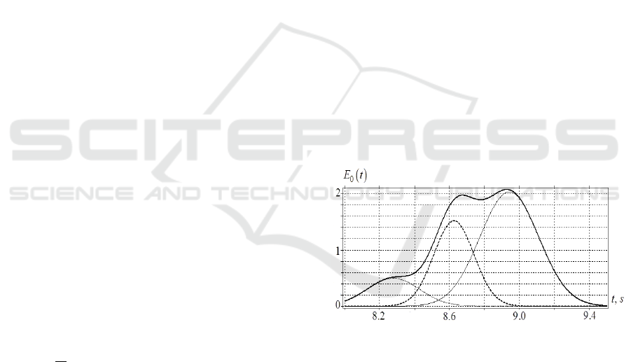
range. To find the minimum (3), we applied the

modified Newton method with accuracy control. The

program was tested on the example of determining

the parameters of Gaussian peaks, when the program

input 𝐸





𝑡



consists of three ideal Gaussian peaks

with the parameters 𝑔⃗







𝑎



;𝑏



;𝑐





(1) close to the

real situation: 𝑔⃗



= (0.49938; 8.2785; 0.15001); 𝑔⃗



(1.5194; 8.6258; 0.11486); 𝑔⃗



= (2.0357; 8.9427;

0.16810). The result of the program is shown in Fig.3.

Analysing this dependence, it is important to note: the

true peaks of the Gaussian curves and the peaks of the

signal 𝐸





𝑡



can occupy different positions in time.

This conclusion will be important in the study of real

records of EEG activity bursts. In addition, a slight

change in the values of 𝑔⃗







𝑎



;𝑏



;𝑐





can

significantly change the topology of the overall

picture 𝐸





𝑡



. The approximation of the system of

nonlinear equations 𝐸







𝑡



using the nonlinear

approximation program (3) reproduces, with

accuracy to the fifth decimal place, the parameters

𝑔⃗



;𝑔⃗



;𝑔⃗



of the test signal 𝐸





𝑡



. The mean square

error between 𝐸







𝑡



and 𝐸





𝑡



is 𝛥  8.3 ⋅ 10



therefore, the curves in Fig.3 merge.

To increase the accuracy of approximation (3), the

experimentally observed values 𝐸





𝐽,𝑡



were

interpolated using the theory of splines. This led to

the fact that the signal sampling step 𝛥𝑡 = 2 ms was

reduced by 20 times. The calculations showed that

most real EEG bursts are satisfactorily described by

three-Gaussian approximation ( 𝑛3), and the

standard deviation between the experimental and

theoretical models is Δ 0.03.

Figure 3: Three Gaussian peaks with the parameters

𝑔⃗



;𝑔⃗



;𝑔⃗



are shown by dots, dashes, and thin lines,

respectively. The bold line corresponds to the sum of three

ideal Gaussian peaks with the parameters𝑔⃗



;𝑔⃗



;𝑔⃗



. The

curve 𝐸





𝑡



and its approximation 𝐸







𝑡



merge entirely into

the bold line.

2.3 Results

2.3.1 Comparison of EEG Simulation

Results and Experimental Data

Let us construct the mathematical model of EEG

burst with the duration [8-9.15 s] in 𝛼 -spectral range,

and follow the change in the shape of this burst while

BIOSIGNALS 2022 - 15th International Conference on Bio-inspired Systems and Signal Processing

moving between two occipital electrodes 𝐽𝑂



→

𝐽𝑂



For the burst in the interval [8-9.15 s], the

difference (3) between the model 𝐸







𝐽,𝑡



and

experimental 𝐸





𝐽,𝑡



is 𝛥



𝑂





 0.024 , and

𝛥



𝑂





 0.027.

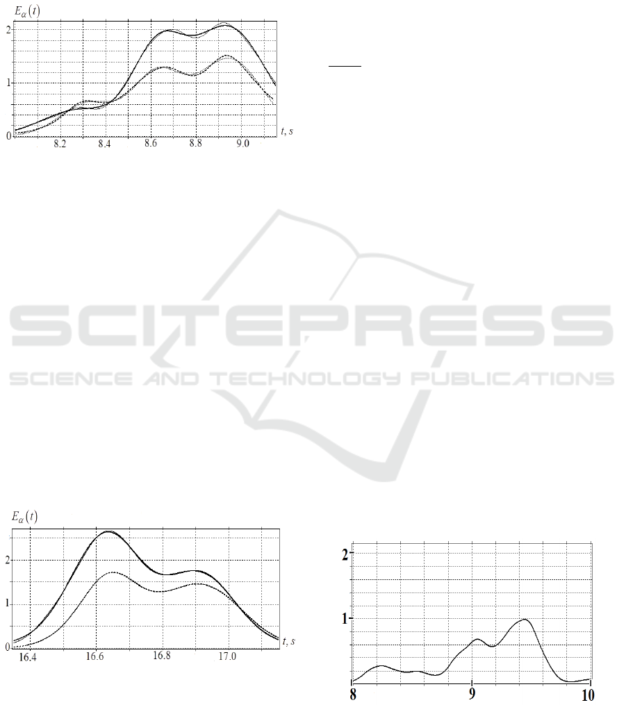
Figure 4: Comparison of the spectral

integrals 𝐸





𝐽,𝑡



obtained for the experimental record of

EEG burst in the interval [8–9.15 s] with their mathematical

models 𝐸





𝐽,𝑡: thin line −𝐸





𝑂



;𝑡



; bold line −𝐸







𝑂



;𝑡



;

dash line −𝐸





𝑂



;𝑡



; dot line −𝐸







𝑂



;𝑡



When the burst propagates in the direction𝑂



→

𝑂



, the behavior of three Gaussian peaks, which form

the model burst in the range [8–9.15 s], is different

(Fig.4). The amplitude of the left peak increases:

𝑎



𝑂



/𝑎





𝑂





= 1.26, the time shift between the

peaks 𝑂



→𝑂



is positive 𝛥𝑡  𝑏





𝑂





𝑏





𝑂





0.0424 s. The amplitude of the central peak decreases

𝑎



𝑂



/𝑎





𝑂





= 0.74. The time shift of the central

peak is negligible 𝛥𝑡  𝑏





𝑂





𝑏





𝑂





= –0.004.

The amplitude of the right peak decreases 𝑎



𝑂



/

𝑎





𝑂





= 0.712, and its maximum lags behind the

maximum of the central peak 𝛥𝑡  𝑏





𝑂





𝑏





𝑂





= 0.0037. The characteristic widths of all three peaks

с



;𝑐



;𝑐



 during their propagation 𝑂



→𝑂



vary

slightly.

Figure 5: Comparison of the spectral integrals

𝐸





𝐽,𝑡



obtained for the experimental record of EEG burst

in the interval [16.2-17.2 s] with their mathematical models

𝐸





𝐽,𝑡: thin line −𝐸





𝑂



;𝑡



; bold line −𝐸







𝑂



;𝑡



; dash

line −𝐸





𝑂



;𝑡



; dot line −𝐸







𝑂



;𝑡



Fig.5 represents the curves 𝐸





𝐽,𝑡



and 𝐸







𝐽,𝑡



for 𝑂



and 𝑂



channels, which correspond to the

burst in the time interval [16.3-17.2 s] (compare with

Fig.4). For such a burst, the agreement between

experiment and theory is better: 𝛥



𝑂





 0.003 ,

𝛥



𝑂





0.02, as compared to that in the interval [8–

9.15 s].

For the burst in the interval [16.2-17.2 s]

propagating in the direction 𝑂



→𝑂



(Fig.5), the

amplitude of the left main peak decreases:

























0.258. The time shift between two main

peaks is positive: 𝛥𝑡  𝑏





𝑂





𝑏





𝑂





=0.007s.

Provided the distance between the nearest (𝑂



→𝑂



)

electrodes 𝐿5cm, the propagation velocity of this

alfa-rhythm peak is 𝑉





𝑂



→𝑂





𝐿/𝛥𝑡, where

𝑉



7.4 ms. Note that the amplitude of the rightmost

peak of this burst increases slightly: 𝑎



𝑂



/

𝑎





𝑂





=1.06. The time shift between the third peaks

during the transition 𝑂



→𝑂



is also positive: 𝛥𝑡 

𝑏





𝑂





𝑏





𝑂





= 0.002 s, and its width becomes

larger 𝑐



𝑂



/𝑐





𝑂





= 1.21. Such an expansion of

the right peak of the burst and a slight increase in its

amplitude can be observed in Fig.5 at time 𝑡  17.1s.

2.3.2 The Trajectories of the EEG Bursts in

α -range and the Map of Cerebral

Cortex Electrical Activity

Let us consider the methodology for calculating the

propagation rates of bursts moving along the cerebral

cortex on the example of EEG bursts in α-range.) We

study two bursts in α-range but in different time

intervals: one evolves in the time interval [8–9.15 s]

(Fig.4), the second in [16.3–17.2 s] (Fig.5). .For each

brain channel, the coordinates of the maximum value

of the spectral integral in the given time interval are

indicated in brackets.

𝐸





𝐽;𝑡



t, s

Figure 6a: Spectral integral in the channel C

(9.444;0.998)

in the interval [8–9.15 s].

Wavelet based Method of Mapping the Brain Activity Waves Travelling over the Cerebral Cortex

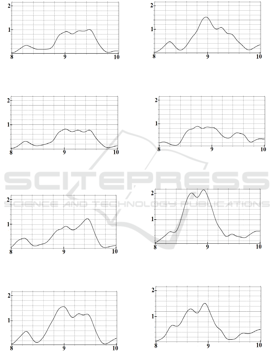
𝐸





𝐽;𝑡



t,s

Figure 6b: Spectral integral in the channel C

(9.456;1.003)

in the interval [8–9.15 s].

𝐸





𝐽;𝑡



t, s

Figure 6c: Spectral integral in the channel C

(9.018;0.815)

in the interval [8–9.15 s].

𝐸





𝐽;𝑡



t, s

Figure 6d: Spectral integral in the channel P

(9.454;1.226)

in the interval [8–9.15 s].

𝐸





𝐽;𝑡



t, s

Figure 6e: Spectral integral in the channel Pz (8.982;1.56)

in the interval [8–9.15 s].

𝐸





𝐽;𝑡



t, s

Figure 6f: Spectral integral in the channel P

(8.970;1.518)

in the interval [8–9.15 s].

𝐸





𝐽;𝑡



t, s

Figure 6g: Spectral integral in the channel 0

(8.724;0.888)

in the interval [8–9.15 s].

𝐸





𝐽;𝑡



t, s

Figure 6h: Spectral integral in the channel 0

(8.920;2.13)

in the interval [8–9.15 s].

𝐸





𝐽;𝑡



t, s

Figure 6i: Spectral integral in the channel 0

(8.934;1.514)

in the interval [8–9.15 s].

BIOSIGNALS 2022 - 15th International Conference on Bio-inspired Systems and Signal Processing

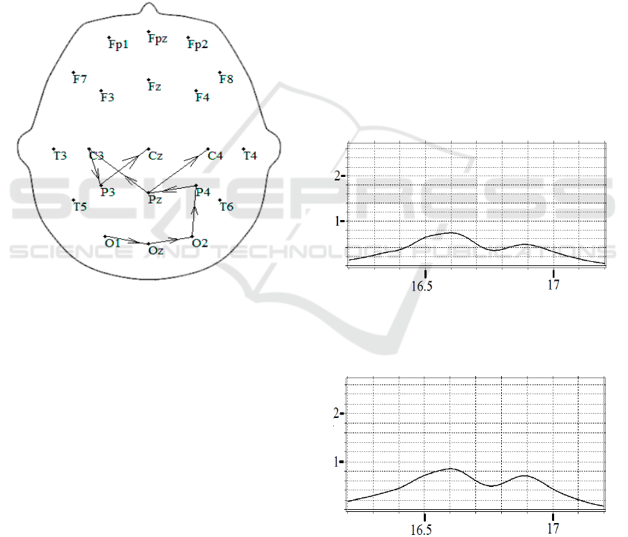
Fig.6 shows the behavior of spectral integrals

𝐸





𝐽;𝑡



in all central channels 𝐽



𝐶



,𝐶



,𝐶



;𝑃



,𝑃



,𝑃



;𝑂



,𝑂



,𝑂





on a single scale in

the interval [8–9.15 s] The development of the burst

during time interval [8–9.15 s] starts in the occipital

channel 𝑂



. Then it reaches a maximum in 𝑂



, and,

gradually decreasing in size, reaches the central

channels 𝑃



and 𝑃



. After that, the burst arrives into

the channel 𝐶



, decreasing in amplitude by 2.6 times

compared with the maximum in 𝑂



. In addition, the

maximum of the burst from the channel 𝑃



moves

along the trajectory 𝐶



→𝑃



→𝐶



(Fig.7). So, the

disturbance spreads from occipital to central and

parietal regions with its activity decreasing in time.

Figure 7: The trajectory of the burst activity maximum in

the time interval [8-9.15 s].

This can be considered as a certain wave process

associated with the excitation of local neural

ensembles caused by some stimuli.

It is important to note that for the peripheral

channels 𝐽𝐹



;𝐹



;𝑇



;𝑇



;𝑇



;𝑇



 the values of

𝐸





𝐽,𝑡



in α-range fall by more than 𝑒  2,72 times

as compared to the maximum value of the burst

observed in the central occipital. The numerical

values 𝐸



𝐽,𝑡





are given for each 𝐽, where 𝑡



is the time moment in seconds at which the maximum

value of the spectral integral for the given channel is

reached. Figures 6 show that the intensities and

shapes of bursts are different for each channel.

Moreover, the maximums of the bursts also vary in

amplitude and time localization, so we may talk about

bursts moving at a certain speed along their own path,

that is, about a wave propagating in a dispersive

medium. The study of Fig.6 makes it possible to find

the trajectories of the maxima of the bursts along the

cerebral cortex. This can be done, if we trace the

maxima of the corresponding spectral integrals in

different channels and connect them.

A different trajectory characterizes the burst in

[16.3-17.2 s] (Fig.8-9). The burst of small amplitude

(0.844) occurs in the central channel 𝐶



. This burst

also reaches its maximum value (2.664) in 𝑂



. A

careful analysis of the shape of the bursts in Fig.4,

Fig.5 shows that an individual burst often has a

complex shape and consists of several peaks. In this

case, the trajectories of the burst maximum do not

take into account the changes in the intensity maxima

redistribution of inside the burst itself. It turns out that

in the case of approximating the total burst 𝐸





𝐽,𝑡



by the mathematical model (2), the velocities,

amplitudes, and widths of each Gaussian peak

appeared to be individual.

The results of calculation of spectral integrals

𝐸





𝐽;𝑡



for different EEG channels in the time

interval [16.3-17.2 s] are shown in Fig.8.

𝐸





𝐽;𝑡



t, s

Figure 8a: Spectral integral in the channel C

(16.600;0,726) in the interval [16.3-17.2 s].

𝐸





𝐽;𝑡



t, s

Figure 8b: Spectral integral in the channel C

(16.602;0,844) in the interval [16.3-17.2 s].

Wavelet based Method of Mapping the Brain Activity Waves Travelling over the Cerebral Cortex

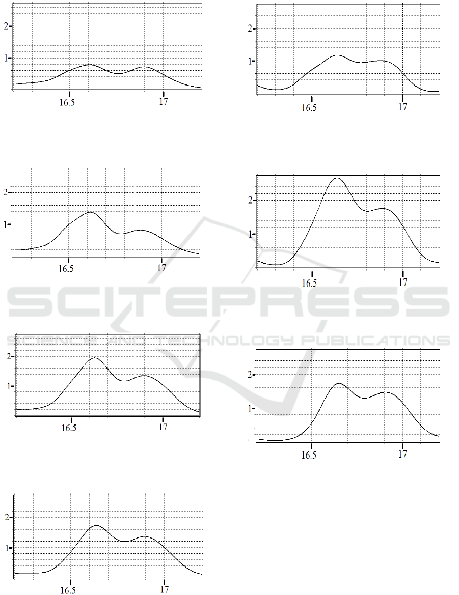
𝐸





𝐽;𝑡



t, s

Figure 8c: Spectral integral in the channel C

(16.606;0,78)

in the interval [16.3-17.2 s].

𝐸





𝐽;𝑡



t, s

Figure 8d: Spectral integral in the channel P

(16.616;1,378) in the interval [16.3-17.2 s].

𝐸





𝐽;𝑡



t, s

Figure 8e: Spectral integral in the channel P

(16.628;1,947)

in the interval [16.3-17.2 s].

𝐸





𝐽;𝑡



t, s

Figure 8f: Spectral integral in the channel P

(16.636;1,722)

in the interval [16.3-17.2 s].

𝐸





𝐽;𝑡



t, s

Figure 8g: Spectral integral in the channel 0

(16.640;1,164)

in the interval [16.3-17.2 s].

𝐸





𝐽;𝑡



t, s

Figure 8h: Spectral integral in the channel 0

(16.638;2,664)

in the interval [16.3-17.2 s].

𝐸





𝐽;𝑡



t, s

Figure 8i: Spectral integral in the channel 0

(16.650;1,721)

in the interval [16.3-17.2 s].

Just like the Figures 6, the Figures 8 show

significant change in intensities and shapes of bursts

in different EEG channels. The maximums of the

bursts also vary in amplitude and time of occurrence,

which indicates the movement of an excitement along

the brain cortex.

BIOSIGNALS 2022 - 15th International Conference on Bio-inspired Systems and Signal Processing

Figure 9: The trajectory of the burst activity maximum in

the time interval [16.3-17.2 s].

2.4 Discussion and Conclusion

In this paper, we propose the mathematical model of

EEG bursts propagating over the cerebral cortex as a

combination of Gaussian peaks with their centers

moving along different trajectories at different

speeds. Each Gaussian peak in the burst is

characterized by its amplitude, maximum in time and

width. In accordance with the nonlinear

approximation model, we approximate each burst by

the sum of three Gaussian peaks with vectors 𝑔⃗







𝑎



;𝑏



;𝑐





, where 𝑖  1,2,3. Calculating the

parameters of each burst makes it possible to

determine changes in the amplitude, shape, direction

of motion, and velocity of the whole burst.

For mapping the movement of bursts over the

cerebral cortex, we used continuous wavelet

transform (CWT) with the Morlet mother wavelet

function, and the temporary analysis of spectral

integrals. By the method of CWT, the spectral

integrals of non-stationary EEG signal have

been calculated for each brain channel 𝐽 in all

frequency ranges 𝜇𝛼,𝛽,𝛾,𝛿. The advantage of

CWT applied in this work over the traditional

window Fourier transform is that the latter requires

the choice of window size 𝑊, which is the additional

problem. For CWT the window size is adjusted

automatically depending on the frequency 𝜈. When

studying signals at low frequencies, the window

becomes wide. In the high-frequency part of the

spectrum (𝛼and 𝛽 rhythms), the window becomes

narrow. In the case when the EEG signal is a

superposition of several non-stationary signals with a

wide spread in characteristic durations and

frequencies, the choice of a single value 𝑊 optimal

for all spectral components 𝜇 may not be possible at

all.

The spectral integrals used in this work

represent the value of the local density of the signal

spectrum integrated over a certain frequency range 𝜇.

An EEG record is presented as some non-stationary

signal − a sequence of bursts, each of which is

characterized by its spectral composition, beginning

and end, and also by the time of electrical activity

maximum. By using the EEG analysis in 𝛼 -range as

an example, it is shown that there are various

scenarios for the appearance and propagation of

bursts in the cerebral cortex. Comparing the

propagation of two bursts, we detected that in one 𝛼 -

burst, an increase in perturbation occurs from the

parietal region of the brain to the occipital. In another

burst, the disturbances spread from the occipital

region. Such a burst fades in the parietal and central

brain channels. Based on the calculation of 𝐸





𝑡



, the

map of activity in those areas of the brain, where the

bursts reach the maximum values, is defined.

In the article (Anodina-Andrievskaya EM et al

2011) on the correlations of various EEG channels at

solving cognitive problems, it was shown that the

correlation map is individual for each person. We

may assume that the map of velocities and directions

of motion (Fig.7, 9) is individual for each person too.

The intensity of the activity bursts and their

localization in time and space recorded in EEG and

ECoEG reflects the spatio-temporal picture of local

neural ensembles reorganization.

The method of tracking the path of the disturbance

propagation over the cerebral cortex can have many

applications. It can be applied in the quantitative

analysis and classification of transients that

characterize the properties of the central nervous

system of a person at the macro level. The method of

restoring the movement of perturbation along the

surface of the brain was used to determine the

dynamics of assimilation and forgetting the rhythm of

photo-stimulation for non-stationary EEG under the

influence of flash. Thus, the mathematical techniques

proposed in the article are the tool for processing

numerous experimental data related to both the

diagnosis of diseases and the study of cognitive

processes in the human brain.

ACKNOWLEDGEMENT

State Task for Basic Research (topic code FSEG-

2020-0024).













Wavelet based Method of Mapping the Brain Activity Waves Travelling over the Cerebral Cortex

REFERENCES

Alexander DM, Jurica P, Trengove C, Nikolaev AR,

Gepshtein S, Zvyagintsev M, Mathiak K, Schulze-

Bonhage A, Ruescher JA, Ball T, Leeuwen C (2013)

Traveling waves and trial averaging: The nature of

single-trial and averaged brain responses in large-scale

cortical signals. NeuroImage, 73, 95–112

Anodina-Andrievskaya EM, Bozhokin SV, Polonsky Yu Z,

Suvorov NB, Marusina MY (2011) Perspective

approaches to analysis of informativity of physiological

signals and medical images of human intelligence.

Journal of instrumental Engineering, 54(7), 27-35

Bahramisharif A, Gerven MAJ, Aarnoutse EJ, Mercier MR,

Schwartz TH, Foxe JF, Ramsey NF, Jensen OJ (2013)

Propagating Neocortical Gamma Bursts Are Coordinated by

Traveling Alpha Waves. Journal of Neuroscience, 33(48),

18849-18854

Belov DR, Kolodyazhnyi SF, Smit NYu (2004) Expression

of Hemispheric Asymmetry and Psychological Type in

the EEG Traveling Wave. Human Physiology, 30(1),

5-19Belov DR, Volnova AV, Ahmediev D(2016)

Travelling wave of ECoG epileptic activity in local

cortical seizure modeling in awake rats. Journal of

Higher Nervous Activity, 66(6), 751-762

Bozhokin SV (2010) Wavelet analysis of learning and

forgetting of photostimulation rhythms for a

nonstationary electroencephalogram. Technical Phys,

55(9), 1248-1256

Bozhokin SV, Suvorov NB (2008) Wavelet analysis of

transients of an electroencephalogram at

photostimulation. Biomed. Radioelectron, N3, 21-25

Bozhokin SV, Suslova IB (2014) Analysis of non-

stationary HRV as a frequency modulated signal by

double continuous wavelet transformation method.

Biomedical Signal Processing and Control, 10, 34-40

Bozhokin SV, Suslova IB (2015) Wavelet-based analysis of

spectral rearrangements of EEG patterns and of non-

stationary correlations. Physica A: Statistical

Mechanics and its Applications, 421(1), 151–160

Bozhokin SV, Zharko SV, Larionov NV, Litvinov AN,

Sokolov IM (2017) Wavelet Correlation of

Nonstationary Signals. Technical Physics, 62(6), 837-

845. https://doi.org/ 10.1134/S1063784217060068

Borisyuk R, Kazanovich Y (2006) Oscillations and waves

in the models of interactive neural populations.

Biosystems, 86, 53-62

Buschman TJ, Denovellis EL, Diogo C, Bullcock D, Miller

EK (2012) Synchronous oscillatory neural ensembles

for rules in the prefrontal cortex. Neuron, 76(1), 838-

846

Getmanenko OV, Belov DR, Kanunikov IE, Smit NY,

Sibarov DA (2006) Reflection of cortical activation

pattern in the human EEG phase structure. Russian

Journal of Physiology, 92(8), 930-948

Chizhov AV, Graham LJ (2008) Efficient evaluation of

neuron populations receiving colored-noise current

based on a refractory density method. Phys.Rev. E, 77,

011910

Gnezditskii VV (2004) A Reverse EEG Problem and

Clinical Electroencephalography. MEDpress-inform,

Moscow

Ivanitsky АМ, Ivanitsky GA, Nikolaev AR, Sysoeva OV

(2009) Encyclopedia of Neuroscience.

Electroencephalography, Springer

Hramov AE, Koronovskii AA, Makarov VA, Pavlov AN,

Sitnikova E (2015) Wavelets in neuroscience. Springer

Series in Synergetics, Springer-Verlag, Berlin,

Heidelberg

Kaplan A, Borisov SV (2003) Dynamic properties of

segmental characteristics of EEG alpha activity in rest

conditions and during cognitive tasks. Zhurnal Vysshei

Nervnoi Deiatelnosti, 53(1), 22-32

Kulaichev AP (2011) The informativeness of coherence

analysis in EEG studies. Neuroscience and behavioral

physiology, 41(3), 321-328

Lopes da Silva F (1991) Neural mechanisms underlying

brain waves: from neural membranes to networks.

Electroenceph. Clin. Neurophysiol, 79, 81–93

Manjarrez E, Vázquez M, Flores A (2007) Computing the

center of mass for traveling alpha waves in the human

brain. Brain Research, 1145, 239 – 247

Massimini M, Huber R, Ferrarelli F, Hill S, Tononi G

(2004) The Sleep Slow Oscillation as a Traveling

Wave. Neurosci., 24(31), 6862– 6870

Muller L, Chavane F, Reynolds J, Sejnowski TJ (2018)

Cortical travelling waves: mechanisms and

computational principles. Nature Reviews

Neuroscience, 19(5), 255–268. https:// doi.org/

10.1038/nrn.2018.20

Mysin IE, Kitchigina VF, Kazanovich YJ (2015)

Modeling synchronous theta activity in the medial

septum: Key role of local communications between

different cell populations. Journal of Computational

Neuroscience, 39, 1-16. https://doi.org/10.1007/

s10827-015-0564-6

Ng V, Barker GJ, Hendler T (2003) Psychiatric

Neuroimaging, Series 1: Life and Behavioural Science,

V.348 of NATO Science Series

Nikolaev AR, Ivanitskii GA, Ivanitskii AM (2001)

Studies of Cortical Interactions over Short Periods of

Time during the Search for Verbal Associations.

Physiology, Neuroscience and Behavioral

Physiology, 31(2), 119-132

Nunez PL (2000) Towads a quantitative description of

large-scale neocortical dynamic function and EEG.

Behavioral and brain sciences, 23, 371–437

Nunez PL, Srinivasan R (2006) Electric Fields of the Brain:

The Neurophysics of EEG, second ed., Oxford

University Press

Ozaki TJ, Sato N, Kitajo K, Someya Y, Anami K, Mizuhara

H, Ogawa S, Yamaguchi Y (2012) Traveling EEG slow

oscillation along the dorsal attention network initiates

spontaneous perceptual switching. Cognitive

Neurodynamics, 6, 185–198

Patten TM, Rennie CJ, Robinson PA, Gong P (2012)

Human Cortical Traveling Waves: Dynamical

Properties and Correlations with Responses. PLoS

ONE, 7(6), e38392

BIOSIGNALS 2022 - 15th International Conference on Bio-inspired Systems and Signal Processing

Pfurtscheller G, Lopes da Silva FH (1999) Event-related

EEG/MEG synchronization and desynchronization:

basic principles. Clinical Neurophysiology, 110, 1842-

1857

Quiles MG, Wang D, Zhaoc L, Romeroc RAF, Huang DS

(2011) Selecting salient objects in real scenes: An

oscillatory correlation model. Neural Networks, 24, 54–

Riedner BA, Vyazovskiy VV, Huber R, Massimini M,

Esser S, Murphy M, Tononi G (2007) Sleep

homeostasis and Cortical Synchronization. III. A high-

density EEG Study of Sleep Slow Waves in Humans.

Sleep, 30(12), 1643-1657

Tafreshi TF, Daliri MR, Ghodousi M (2019) Functional and

effective connectivity-based features of EEG signals

for object recognition. Cognitive Neurodynamics,

13(6), 555-566

Trofimov AG, Kolodkin IV, Ushakov LV, Velichkovsckii

BM (2015) Agglomerative method for isolating

microstates EEG related to the characteristics of the

traveling wave. Neuroinformatic-2015, MIFI, Moscow,

Part 1. P. 66-77

Terman DH, Ermentrout GB, Yew AC (2001) Propagating

activity patterns in thalamic neuronal networks. SIAM

Journal on Applied Mathematics, 61, 1578–1604

Tong S, Thakor NN (2009) Quantitative EEG Analysis

Methods and Clinical Applications. Artech House.

Boston. London

Verkhlyutov VM, Balaev VV, Ushakov VL, Velichkovsky

BM (2019) A Novel Methodology for Simulation of

EEG Traveling Waves on the Folding Surface of the

Human Cerebral Cortex. Studies in Computational

Intelligence, 799, 51-63. https://doi.org/10.1007/978-3-

030-01328-8_4

Villacorta-Atienza JA, Makarov VA (2013) Wave-

Processing of Long-Scale Information by Neuronal

Chains. PLoS ONE 8(2), e57440.

https://doi.org/10.1371/journal.pone.0057440

Voytek B, Canolty R, Shestyuk A, Crone N, Parvizi J,

Knight R (2010) Shifts in gamma phase–amplitude

coupling frequency from theta to alpha over posterior

cortex during visual tasks. Frontiers in Human

Neuroscience, 4, 191

Zenkov LR (2013) Clinical Electroencephalography,

MEDpress-inform

Zhang H, Watrous AJ, Patel A, Jacobs J (2018) Theta and

alpha oscillations are traveling waves in the human

neocortex. Neuron, 98(6), 1269-1281. https://doi.org/

10.1016/j.neuron.2018.05.019

Wavelet based Method of Mapping the Brain Activity Waves Travelling over the Cerebral Cortex