Heart Rate Estimation based on Optical Flow: Enabling Smooth Angle

Changes in Ultrasound Simulation

Henning Sch

afer

1,2 a

, Hendrik Damm

1,3 b

and Christoph M. Friedrich

1,4 c

Department of Computer Science, University of Applied Sciences and Arts Dortmund (FHDO), Dortmund, NRW, Germany

Institute for Transfusion Medicine, University Hospital Essen, Essen, NRW, Germany

Institute of Epidemiology and Social Medicine, University of M

unster, M

unster, NRW, Germany

Institute for Medical Informatics, Biometry and Epidemiology (IMIBE), University Hospital Essen, Essen, NRW, Germany

Keywords:

Biomedical Image Processing, Ultrasound Imaging, Vascular Imaging, Image Visualization, Functional Image

Analysis, 3D Video-based Ultrasound Simulation.

Abstract:

Ultrasound simulators show previously recorded ultrasound videos from different angles to the trainee. During

acquisition, breathing, pulse, and other motion artifacts are involved, which often prevent a smooth image

transition between different angles during simulation. In this work, a global motion vector is derived using

the Lucas–Kanade method for calculating the optical ﬂow in order to create a motion proﬁle in addition to the

recording. This proﬁle allows transition synchronization in ultrasound simulators. For the transition in kidney

recordings, the Pearson’s r correlation could be increased from 0.252 to 0.495 by autocorrelating motion

proﬁles and synchronizing them based on calculated delays. Approaches based on tracking and structural

similarity were also evaluated, yet these have shown inferior qualitative transition results. In ultrasound videos

with visibility of vessels, e.g., thyroid gland with carotid artery or echocardiogram, the heart rate can also be

estimated via the optical ﬂow. In the abdominal region, the signal contains respiratory information. Since the

motion proﬁle can be generated in real time directly at the transducer position, it could be useful for diagnostic

purposes.

1 INTRODUCTION

An ultrasound simulator is a medical simulation train-

ing device that enables trainees to practice diagnos-

tic, therapeutic, and surgical applications related to

ultrasound-based imaging techniques. To achieve

these training results, simulators mimic the ultra-

sound image. An ultrasound simulator, 3D video-

based, shows previously recorded ultrasound videos

from different angles. When the trainee moves the

transducer, e.g., an imitation with a gyroscope sensor,

transitions should be made between the recordings

from the different angles so that a realistic scenario

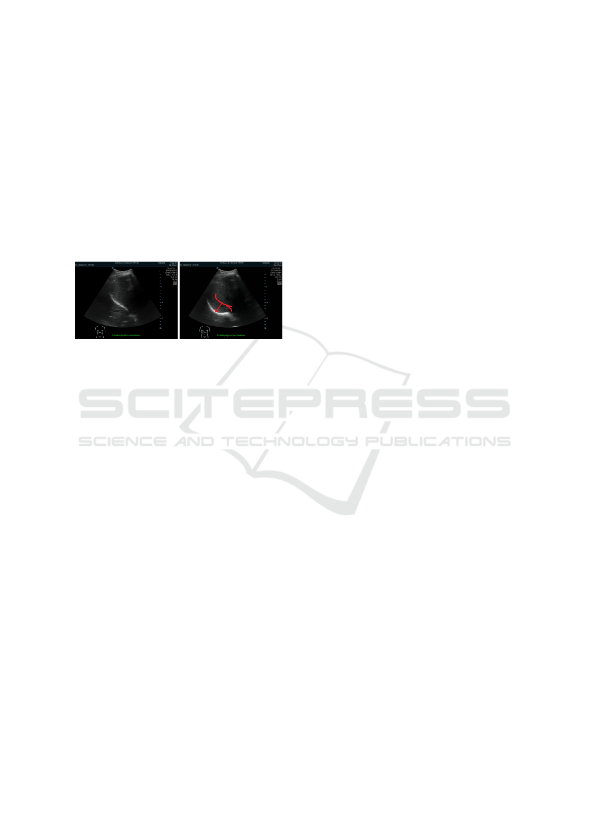
of the sounding of an organ can be reproduced. Dur-

ing angle transition, hard image jumps can occur (see

Figure 1). This is because of respiration, pulse, and

other motion artifacts that were recorded at the time of

acquisition. Here, a structures to be observed jumps

https://orcid.org/0000-0002-4123-0406

https://orcid.org/0000-0002-7464-4293

https://orcid.org/0000-0001-7906-0038

further (see previous position based on red line), be-

cause the asynchronous angle change causes the res-

piration to be in a different cycle. In order to pre-

vent these jumps during simulation, a synchronization

of the recordings from the different angles is needed.

The objective of this work is to apply and evaluate

different methods to investigate their suitability for

synchronizing ultrasound acquisitions from different

angles. An overview on other approaches for ultra-

sound simulators can be seen in (Ourahmoune et al.,

2012; Blum et al., 2013). Starting from an arbitrary

frame of one angle, the best matching frame from the

target angle is to be selected, so that there are mini-

mal artifacts as possible during transition. Both an-

gles need to be synchronized with respect to respi-

ration and pulse. Previous approaches to synchro-

nize the images by recording the respiration and the

pulse could not always enable a smooth change. The

abdominal region, where vascular and thoracic res-

piratory motion affect the ultrasound image, is con-

sidered to be challenging. For this work, videos of or-

gans were acquired at different angles. These are each

236

Schäfer, H., Damm, H. and Friedrich, C.

Heart Rate Estimation based on Optical Flow: Enabling Smooth Angle Changes in Ultrasound Simulation.

DOI: 10.5220/0010902000003123

In Proceedings of the 15th International Joint Conference on Biomedical Engineering Systems and Technologies (BIOSTEC 2022) - Volume 4: BIOSIGNALS, pages 236-243

ISBN: 978-989-758-552-4; ISSN: 2184-4305

10 seconds long and have a frame count of 30 frames

per second. They are to be displayed to the trainee in

a continuous loop to simulate a real ultrasound image.

A transducer mockup with a gyroscope is used to esti-

mate its angle for selection of the respective imaging

output from recordings. In the case of a change of an-

gle, transitions occur, which are to be synchronized by

means of different approaches, which are presented in

this work.

In the remainder of this paper, Section 2 provides

a short overview of related work and state of the art

approaches. Section 3 describes the methods used in

this paper. In Section 4 the obtained results are evalu-

ated and ﬁnally concluded afterwards in Section 5.

(a) Kidney 90 degrees (b) Kidney 95 degrees

Figure 1: Transition through a kidney examination, (a)

shows imaging output at 90°, (b) shows imaging output at

95° with a motion artifact due to respiration (marked in red).

2 RELATED WORK

This section describes related work used for synchro-

nization approaches.

2.1 Optical Flow

Optical ﬂow is a commonly used method for mo-

tion estimation in a scene with a wide range of ap-

plications. Many gradient-based methods such as the

Horn-Schunck method (Horn and Schunck, 1981) and

the Lucas-Kanade method (Lucas and Kanade, 1981)

have been developed to estimate optical ﬂow based on

the calculation of brightness gradients.

In the gradient-based methods, partial derivatives

with respect to temporal coordinates are calculated

as brightness gradients (Kearney et al., 1987). As

soon as objects in a scene move with high velocities,

the gradient-based methods are less suitable (Lawton,

1983). Gradient-based optical ﬂow methods, unlike

correlation-based ﬂow methods (Bergen et al., 1990;

Lawton, 1983) can be computed more quickly and

are suitable for real-time estimation of optical ﬂow.

The Lucas-Kanade method is a widely used differ-

ential method for estimating optical ﬂow proposed

by Bruce D. Lucas and Takeo Kanade (Lucas and

Kanade, 1981). It assumes that the optical ﬂow in the

neighborhood of the pixel is a constant, and then uses

the least squares method to solve the basic equation

of optical ﬂow for all pixels in the neighborhood.

2.2 Structural Similarity

From a study on tracking in ultrasound images of the

tongue (Xu et al., 2016), the Complex Wavelet Struc-

tural Similarity Index (CW-SSIM) behaves uniformly

and predictably for slight rotations in ultrasound im-

ages. To this end, different metrics for calculating

similarity were compared for rotations ranging from

-10°to 10°+ in an ultrasound image.

The Structural Similarity Index (SSIM) is a

method for measuring the similarity between two im-

ages (Wang et al., 2004). The index is often under-

stood as a quality measure against the image to be

compared, e.g. altered by noise.

The metric is based on the assumption that the hu-

man visual system (HVS) model is more responsive to

structural changes. Therefore, a measure that quanti-

ﬁes structural similarity should be a good approxima-

tion of the actual changes perceived by the HVS.

The CW-SSIM index (Sampat et al., 2009) is an

extension of the SSIM to the complex wavelet do-

main, which is more robust to certain image changes

(e.g., translation and rotation).

2.3 Tracking

During the tracking approach, various frames of an

angle should be downstreamed at random intervals to

verify that tracking of the structure continues. The

assumption is that if the tracking of a structure can be

continued successfully, there is a smooth change of

angle.

The Discriminative Correlation Filter with Chan-

nel and Spatial Reliability (DCF-CSR) is a tracking

method for short-term tracking of structures (Bolme

et al., 2010; Luke

c et al., 2018). Here, tracking

using Correlation Filter has been extended to DCF

tracking by the concepts of channel and spatial reli-

ability. Spatial reliability adjusts ﬁlter support to the

region of the object selected for tracking. This allows

both an increase in search area and better tracking of

non-rectangular objects (Luke

c et al., 2018).

With only two features, histogram of oriented gra-

dients (HoGs) and colornames, the CSR-DCF method

achieves state-of-the-art results on several tracking

challenges (VOT 2016, VOT 2015, and OTB100)

(Matej et al., 2016; Roffo et al., 2016; Wu et al.,

2015). The CSR-DCF runs in real-time on a CPU.

Heart Rate Estimation based on Optical Flow: Enabling Smooth Angle Changes in Ultrasound Simulation

237

2.4 Heart Rate Estimation

One way of enriching the ultrasound images with fur-

ther information is to indicate the heart rate. If this

was not recorded at the time of acquisition, it can

be reconstructed by visual image processing. Theo-

retically, this possibility exists whenever image areas

of the ultrasound are directly or indirectly exposed

to changes caused by the expansion of blood vessels.

Puybareau et al. (Puybareau et al., 2015) use ﬁsh em-

bryos to show that the optical ﬂow of blood vessels in

the heart can be used to reconstruct the pulse. Further-

more, a distinction between artery and vein could be

derived from clustering of the speed vectors. Bouk-

erroui et al. (Boukerroui et al., 2003) show that the

movement of the endocardium (innermost layer of the

heart wall) in the left ventricle can be tracked based

on ultrasound images using velocity estimation. The

movements of the left ventricle were recorded over

time similar to the tracking of ﬁsh embryo vessels

(Puybareau et al., 2015).

3 METHODS

The approaches described in Section 2, namely op-

tical ﬂow (see Section 3.1), CW-SSIM (see Section

3.3), and tracking with DCF-CSR (see Section 3.2),

will be applied to different ultrasound recordings. For

this purpose, videos of the kidney, thyroid and differ-

ent views of the heart (echocardiography)

, as well

as the abdomen (gallbladder) will be used. Except

for the cardiac ultrasound, all recordings for this work

were acquired in 30 FPS and are always 10 seconds

long

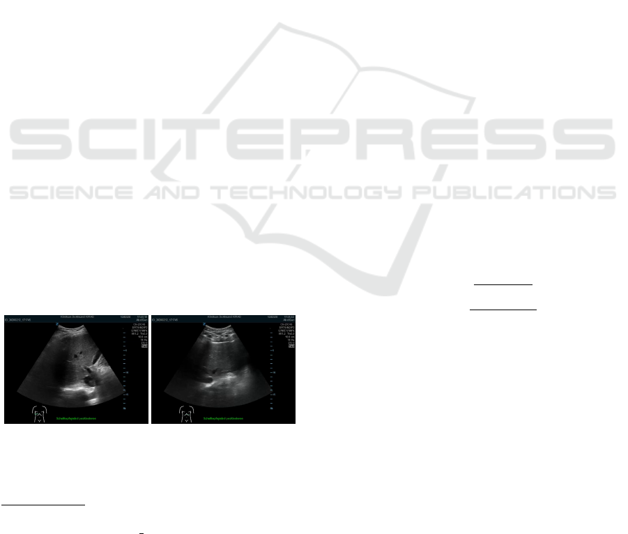
. For each image, there is a corresponding angle

spectrum from approximately -30° to +30° in 5° de-

gree steps (see Figure 2).

(a) Kidney (b) Gallbladder

Figure 2: (a) Image of the kidney with structures partially

moving due to pulse and respiration, (b) Image of the gall-

bladder with movement of the abdomen due to respiration.

Echocardiography views were taken from

https://youtu.be/2XR6etAY -w, last accessed: 07.11.2021

Acquired from ZONARE ZS3, C6-2, convex trans-

ducer, 2-6 MHz.

3.1 Optical Flow Calculation via

Lucas–Kanade

The Lucas-Kanade method is used to approximate the

optical ﬂow. For this purpose, the original image is

divided into smaller sections. The basic calculation

of the algorithm (Lucas and Kanade, 1981; Ishii et al.,

2011) is shown in equation (1).

+ υ

= 0 (1)

I(x, y,t) describes the brightness of a pixel at po-

sition (x,y) at time t. If I(x,y,t) does not change ex-

cessively between frames, the optical ﬂow can be cal-

culated using equation (1), where I

, I

and I

are the

partial derivatives of I(x,y,t) resolved to x, y and t. υ

and υ

describe the velocity, i.e., the momentum of

motion associated with the optical ﬂow of I(x,y,t). It

is now assumed that υ

and υ

remain constant over

a smaller range, from which equation (2) is derived

(Ishii et al., 2011).

+ S

= 0

+ S

= 0

(2)

Where S

, S

and S

are the product

sums of the partial derivatives of I

, I

and I

in the

costant small range Γ (shown in equation (3)) (Ishii

et al., 2011).

∑

y =

∑

(3)

The velocity in x and y direction can be calculated

by solving equation (2) over equation (4) (Ishii et al.,

2011).









−S





(4)

By using the velocity vectors υ

, υ

the move-

ment of pixels with constant brightness of a region

is obtained. Since in ultrasound images the inten-

sity of structures does not change much and there-

fore strong jumps are not to be expected, the Lucas-

Kanade method is considered to be suitable for esti-

mating optical ﬂow.

3.1.1 Global Motion Proﬁle Generation via

Lucas–Kanade

In order to smoothly change the angle between the

recordings of an organ at any frame, a global motion

proﬁle is to be generated. For this purpose, the veloc-

ity of a zone is calculated for each frame in compari-

son to the previous frame.

BIOSIGNALS 2022 - 15th International Conference on Bio-inspired Systems and Signal Processing

238

To optimize the calculation, the image is divided

into 8 × 8 zones. The size of the zone depends on

the resolution of the ultrasound recording. Since the

motion proﬁle can be preprocessed for the transitions,

small zones at high resolution are also possible. Here,

the distribution of apparent velocities in direction u

and v yields an average movement of brightness pat-

tern D (Du

and Dv

) of a 8 × 8 pixel zone at time

The idea for motion proﬁling is now based on the

fact that the average of all movements within a frame

gives a global motion tendency DG of the optical ﬂow

(DG

and DG

) (see equation (5)), where k stands for

the number of all 8× 8 regions in an ultrasound frame.









∑





(5)

The global movement of brightness DG

and DG

measured over the duration of the recording gives the

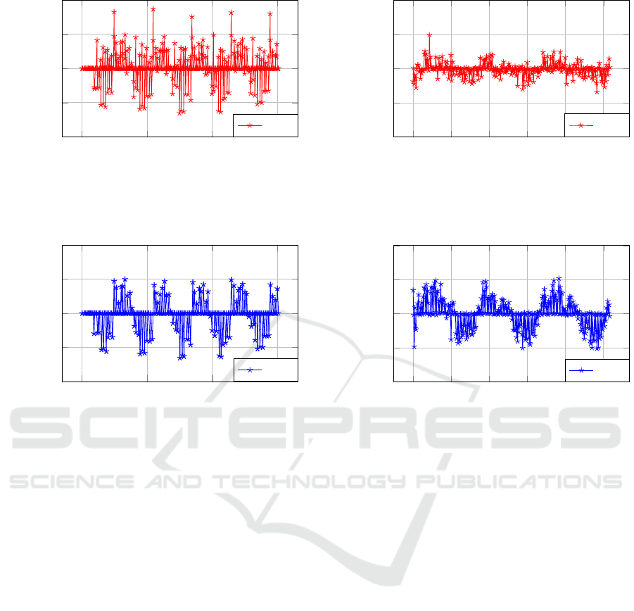
motion proﬁle of an ultrasound video. Figure 3 shows

such a motion proﬁle to an echocardiogram recorded

over 3 seconds of DG in the direction u, the movement

on the horizontal axis. Figure 4 shows DG in the v

direction, the movement on the vertical axis.

3.1.2 Heart Rate Estimation via Global Motion

Proﬁles

To estimate the heart rate from a raw optical ﬂow sig-

nal, the Pan-Tompkins method (Pan and Tompkins,

1985) is used. The Pan-Tompkins method applies a

series of ﬁlters to emphasize the frequency content of

the cardiac depolarization.

The values determined by optical ﬂow are the ve-

locity values in m/s from equation (5). Due to the

adaptive threshold, the algorithm should still be able

to reliably detect an edge from the raw signal, pro-

vided that a vessel is recorded.

3.2 Discriminative Correlation Filter

with Channel and Spatial Reliability

Tracking of structures is also a possible approach to

prevent image jumps during changeover. The struc-

tures changing due to respiration and pulse over the

period of the ultrasound recording could be recog-

nized in the frames of the recording of the next angle.

Here, out of all the frames in which tracking can

be continued, the frame with the smallest distance of

the tracked area from the original frame is assumed

to achieve a continuation of the natural motion. The

opencv (Bradski, 2000) implementation was used.

3.3 Complex Wavelet Structural

Similarity

For this method, a random frame was taken from the

recordings of a kidney (source frame) and compared

with all possible frames in the next angle of the ul-

trasound recording using the Similiarity Index (CW-

SSIM).

4 EVALUATION

The presented methods have been evaluated with re-

spect to their suitability for smooth angle changes in

ultrasound simulators.

4.1 Optical Flow

To enable synchronized angle changes, the optical

ﬂow motion proﬁles of different angles on ultrasound

images of a same organ are assumed to be signals that

correlate with themselves at an earlier time. These re-

current movements, e.g., due to respiration, can there-

fore be synchronized by determining the lag to an ad-

jacent angle.

For example, in the ultrasound simulator the

recording is permanently shown from angle 90 de-

grees. If the trainee decides to change the view to

95 degrees, the lag is resolved via autocorrelation

(Bracewell, 1978), resulting in a synchronous change.

For this purpose, the lag to the pre-signal is compen-

sated and the result is translated into the appropriate

frame on the time axis, so that the new image contin-

ues e.g. at the same time of the breathing phase. The

synchronization of the angle changes by the motion

proﬁles in horizontal and vertical direction by means

of shifting the lag was tested by carrying out angle

changes at random time, in each case with and with-

out synchronization. Without synchronization, struc-

tures of the ultrasound image suddenly appear at other

positions after the change, because they have shifted

at the time of acquisition, e.g. due to respiration or

pulse. Such a jump can be seen in Figure 1. With

synchronization, it is also clearly visible that the an-

gle has changed, but the moving structures to be ob-

served are continued in their movement, resulting in a

smooth change.

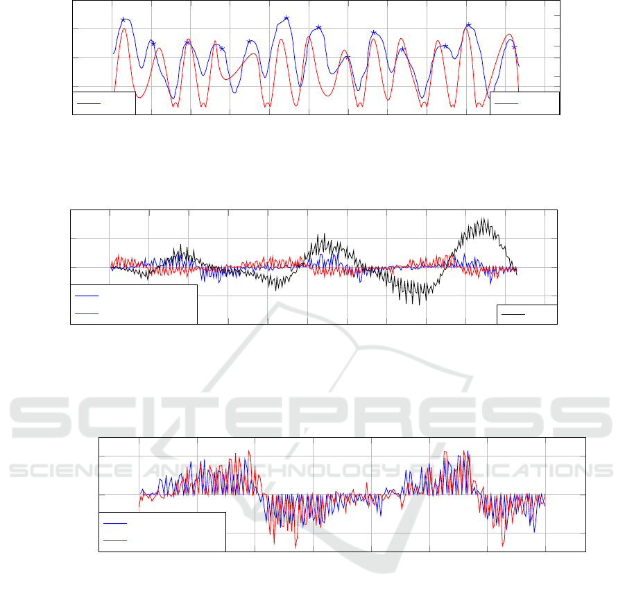
The application of the signals of two angles

aligned by the determined lag through autocorrelation

(see Figure 8) can be seen in Figure 9. After shifting

by the compensated lag, these result in a synchronized

motion proﬁle. To ensure that the motion proﬁle con-

tain valuable information, proﬁles of recordings with

Heart Rate Estimation based on Optical Flow: Enabling Smooth Angle Changes in Ultrasound Simulation

239

0 1 2 3

−1

−0.5

0.5

time (s)

velocity(m/s)

Figure 3: Global movement DG as velocity (m/s) in direc-

tion u (horizontal axis) determined in an echocardiogram

measured over time (s).

0 1 2 3

−1

−0.5

0.5

time (s)

velocity(m/s)

Figure 4: Global movement DG as velocity (m/s) in di-

rection v (vertical axis) determined in an echocardiogram

measured over time (t).

movements through vessels as well as through res-

piration were generated. Figure 3 shows the global

movement DG as velocity (m/s) in direction u (hor-

izontal axis) determined in an echocardiogram mea-

sured over time (t). Figure 4 shows the recording cor-

respondingly in vertical axis. The 3-second recording

is from the coronary venous sinus view of the heart.

Here, the heart rate of 5 beats in 3 seconds is visible

on both axes and can be read visually. The motion

proﬁle could also be interpreted well in other views

such as the full view (four chamber view) or the mi-

tral valve.

For organs in the abdominal region, such as the

gallbladder, the expansion of the thorax due to respi-

ration is the main factor for movements in the ultra-

sound image. Figure 5 shows the global movement

DG in horizontal axis determined in the abdomen

(gallbladder) measured over a period of about 10 sec-

onds. Here, the motion is not visible because the ac-

quisition was horizontal and therefore the respiratory

motion is mainly in the direction of the vertical axis.

Figure 6 shows the global movement DG in verti-

cal axis. The respiratory cycle can be read well. In the

period of 10 seconds, 3 respiratory cycles took place.

0 2 4

8 10

−0.4

−0.2

0.2

0.4

time (s)

velocity(m/s)

Figure 5: Global movement DG as velocity (m/s) in direc-

tion u (horizontal axis) determined in the abdomen (gall-

bladder) measured over time (s).

0 2 4

8 10

−0.4

−0.2

0.2

0.4

time (s)

velocity(m/s)

Figure 6: Global movement DG as velocity (m/s) in direc-

tion v (vertical axis) determined in the abdomen (gallblad-

der) measured over time (s). Here visible, the 3-fold respi-

ratory cycle.

4.1.1 Heart Rate Estimation

Figure 7 shows the estimation of heart rate with the

Pan-Tompkins method (blue markers). Here, an ultra-

sound video of the aorta was used to determine optical

ﬂow.

The optical ﬂow was smoothed with a Gaussian

ﬁlter and then overlaid with data obtained from a

pulse oximeter worn on the left index ﬁnger. The

pulse was recorded synchronously in addition to the

optical ﬂow during ultrasound acquisition. The opti-

cal ﬂow and the pulse curve correlate with each other.

The adaptive threshold allows the algorithm to

perform edge detection from the raw signal and es-

timate the heart rate by counting detected peaks, pro-

vided a vessel is recorded.

4.2 Tracking with DCF-CSR

For this experiment, several images of the kidney

were chosen with smaller artifacts that change with

respiration and/or pulse. During tracking, different

frames of an applied angle were then downstreamed

BIOSIGNALS 2022 - 15th International Conference on Bio-inspired Systems and Signal Processing

240

−1 0 1 2 3 4

5 6

7 8 9 10 11

−1

−0.5

0.5

200

400

600

time (s)

velocity(m/s)

pulse oxi(nm)

pulse

Figure 7: Estimation of heart rate using Pan-Tompkins method on the raw signal of the motion proﬁle and the pulse oximeter

for validation (in this case, ultrasound of the aorta on the vertical axis).

0 1 2 3 4

5 6

7 8 9 10 11

−1

−0.5

0.5

−1

−0.5

0.5

time (s)

velocity(m/s)

correlation

Kidney 90

◦

Kidney 95

◦

corr

Figure 8: Vertical motion proﬁles of ultrasound recordings of the kidney at two different angles and the corresponding cross-

correlation. A lag of 3 seconds in the respiratory cycle at the two angles results from the different start times of the ultrasound

acquisition and can be seen in the motion proﬁle here. Pearson r correlation coefﬁcient between both angles (without resolving

lag) is 0.252.

3 4

5 6

7 8 9 10

−0.2

0.2

time (s)

velocity(m/s)

Kidney 90

◦

Kidney 95

◦

Figure 9: Synchronized motion proﬁle, shifted over lag determined by autocorrelation. By compensating for lag, the moving

structures to be observed are continued in their movement. In this example, pearson r correlation increases from 0.252 to

0.4953 by synchronizing the lag.

at randomly selected intervals to check whether the

tracking of the structure can be continued.

Since the search range in DCF-CSR is very high,

errors often occured and another structure was contin-

ued. Tracking beyond the angle change is error-prone,

as the object may no longer be visible. The carotid

artery near the thyroid gland could be tracked well,

but not with sufﬁciently high FPS. Accordingly, the

tracking would have to be preprocessed.

This approach also lacks the tendency of the

movement, i.e. the position of the object can be at

the same place e.g. when exhaling and inhaling with

a different momentum each time, but this is not con-

sidered in the search range of the tracking in the new

angle.

4.3 Frame Comparison with CW-SSIM

For this experiment, a random frame was taken from

the image of a kidney (source frame) and compared

with all possible frames in the next angle of the ultra-

sound image using the Similiarity Index (CW-SSIM).

The structure of interest moved horizontally during

the acquisition, so it is necessary to ﬁnd a frame that

Heart Rate Estimation based on Optical Flow: Enabling Smooth Angle Changes in Ultrasound Simulation

241

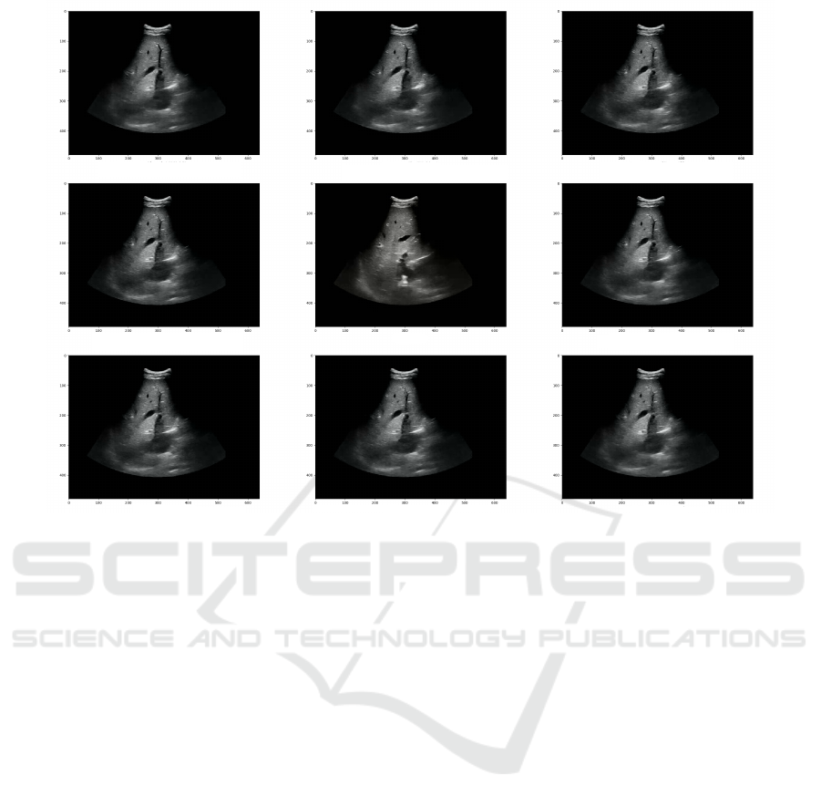
Frame18 CW_SSIM: 0.8223

Frame44 CW_SSIM: 0.8213 Frame29 CW_SSIM: 0.8180

Frame28 CW_SSIM: 0.8177

Frame23 CW_SSIM: 0.8172

Frame34 CW_SSIM: 0.8165 Frame26 CW_SSIM: 0.8160

Frame37 CW_SSIM: 0.8159

Source Frame

Figure 10: The highest CW-SSIM values compared to the source frame (angle prior to transition) at the +10°angle of the

abdomen.

shows the structure on a similar position of the X-axis

to allow a smooth change.

Figure 10 shows the 8 frames in the target angle

with the highest CW-SSIM values compared to the

source frame.

The frames with the smallest change in the

+10°degree step of the kidney are all from a similar

similarity range. Structural similarity can be appro-

priate, but would need to be preprocessed (n × m pos-

sibilities in each of the two angular directions).

Another drawback analogous to the tracking prob-

lem is the lack of momentum. In the case of the respi-

ration curve, there are several similar CW-SSIM val-

ues at the time of inhalation or exhalation, which, un-

like optical ﬂow, cannot be distinguished.

5 CONCLUSION

In this work, three systems were presented and eval-

uated for their suitability for smooth angle change in

ultrasound simulators. The calculation of the motion

proﬁle using optical ﬂow proved to be successful and

can be integrated into simulators. The angle transition

is expected to be synchronous in the abdomen as well

as with visibility of vessels and is preferable to pre-

vious synchronization based on respiratory and pulse

recordings at the time of acquisition, since both arti-

facts are taken into account.

For future work, the proposed method should be

evaluated based on explicit quality criteria and on

additional organs. Since ultrasound simulators are

rarely open source, it is difﬁcult to directly compare

the proposed method with other approaches side by

side. Therefore, in the future, there should be ef-

forts to provide an open source ultrasound simula-

tor in which this method can then be applied along-

side others. In addition, it would be useful to publish

some recordings to generate a benchmark dataset for

synchronization of ultrasound recordings. It should

also be investigated whether the motion proﬁles can

be useful for diagnostic purposes besides estimating

heart rate and respiratory rate.

REFERENCES

Bergen, J. R., Burt, P. J., Hingorani, R., and Peleg, S.

(1990). Computing two motions from three frames.

In International Conference on Computer Vision, vol-

ume 90, pages 27–32.

Blum, T., Rieger, A., Navab, N., Friess, H., and Martignoni,

M. (2013). A review of computer-based simulators for

ultrasound training. Simulation in Healthcare, 8(2).

Bolme, D. S., Beveridge, J. R., Draper, B. A., and Lui, Y. M.

BIOSIGNALS 2022 - 15th International Conference on Bio-inspired Systems and Signal Processing

242

(2010). Visual object tracking using adaptive correla-

tion ﬁlters. In 2010 IEEE computer society conference

on computer vision and pattern recognition (CVPR),

pages 2544–2550. IEEE.

Boukerroui, D., Noble, J. A., and Brady, M. (2003). Veloc-

ity estimation in ultrasound images: A block match-

ing approach. In Biennial International Conference

on Information Processing in Medical Imaging, pages

586–598. Springer.

Bracewell, R. (1978). The Fourier Transform and its Appli-

cations. McGraw-Hill Kogakusha, Ltd., Tokyo, sec-

ond edition.

Bradski, G. (2000). The opencv library. Dr. Dobb’s Journal

of Software Tools, 25:120–125.

Horn, B. K. and Schunck, B. G. (1981). Determining op-

tical ﬂow. In Techniques and Applications of Image

Understanding, volume 281, pages 319–331. Interna-

tional Society for Optics and Photonics.

Ishii, I., Taniguchi, T., Yamamoto, K., and Takaki, T.

(2011). High-frame-rate optical ﬂow system. IEEE

Transactions on Circuits and Systems for Video Tech-

nology, 22(1):105–112.

Kearney, J. K., Thompson, W. B., and Boley, D. L. (1987).

Optical ﬂow estimation: An error analysis of gradient-

based methods with local optimization. IEEE Trans-

actions on Pattern Analysis and Machine Intelligence,

PAMI-9(2):229–244.

Lawton, D. T. (1983). Processing translational motion se-

quences. Computer Vision, Graphics, and Image Pro-

cessing, 22(1):116–144.

Lucas, B. D. and Kanade, T. (1981). An iterative image

registration technique with an application to stereo vi-

sion. In Proceedings of the 7th International Joint

Conference on Artiﬁcial Intelligence - Volume 2, IJ-

CAI’81, page 674–679, San Francisco, CA, USA.

Morgan Kaufmann Publishers Inc.

Luke

c, A., Voj

r, T.,

Cehovin Zajc, L., Matas, J., and

Kristan, M. (2018). Discriminative correlation ﬁlter

tracker with channel and spatial reliability. Interna-

tional Journal of Computer Vision, 126(7):671–688.

Matej, K. et al. (2016). The visual object tracking vot2016

challenge results. In European Conference on Com-

puter Vision (ECCV) Workshops.

Ourahmoune, A., Larabi, S., and Hamitouche-Djabou, C.

(2012). A survey of echographic simulators. In Gi-

amberardino, P. D., Iacoviello, D., Tavares, J. M.

R. S., and Jorge, R. M. N., editors, Computational

Modelling of Objects Represented in Images - Fun-

damentals, Methods and Applications III, Third Inter-

national Symposium, CompIMAGE 2012, Rome, Italy,

September 5-7, 2012, pages 273–276. CRC Press.

Pan, J. and Tompkins, W. J. (1985). A real-time qrs de-

tection algorithm. IEEE transactions on biomedical

engineering, BME-32(3):230–236.

Puybareau, E., Talbot, H., and L

eonard, M. (2015). Auto-

mated heart rate estimation in ﬁsh embryo. In 2015

International Conference on Image Processing The-

ory, Tools and Applications (IPTA), pages 379–384.

IEEE.

Roffo, G., Kristan, M., Matas, J., Felsberg, M., Pfugfelder,

R., Cehovin, L., Vojjir, T., Hager, G., Melzi, S., and

Fernandez, G. (2016). The visual object tracking

vot2016 challenge results. In Proceedings of the IEEE

European Conference on Computer Vision Workshops

(ECCV), Amsterdam, The Netherlands, pages 8–16.

Sampat, M. P., Wang, Z., Gupta, S., Bovik, A. C., and

Markey, M. K. (2009). Complex wavelet structural

similarity: A new image similarity index. IEEE trans-

actions on image processing, 18(11):2385–2401.

Wang, Z., Bovik, A. C., Sheikh, H. R., and Simoncelli, E. P.

(2004). Image quality assessment: from error visi-

bility to structural similarity. IEEE transactions on

image processing, 13(4):600–612.

Wu, Y., Lim, J., and Yang, M. (2015). Object tracking

benchmark. IEEE Transactions on Pattern Analysis

and Machine Intelligence, 37(9):1834–1848.

Xu, K., G

abor Csap

o, T., Roussel, P., and Denby, B. (2016).

A comparative study on the contour tracking algo-

rithms in ultrasound tongue images with automatic re-

initialization. The Journal of the Acoustical Society of

America, 139(5):EL154–EL160.

Heart Rate Estimation based on Optical Flow: Enabling Smooth Angle Changes in Ultrasound Simulation

243