
Visual Tilt Correction for Vehicle-mounted Cameras
Firas Kastantin and Levente Hajder
Department of Algorithms and their Applications, E
¨
otv
¨
os Lor
´
and University,
P
´
azm
´
any P
´
eter stny. 1/C, Budapest 1117, Hungary
Keywords:
Camera Tilt Correction, Planar Motion, Vehicle-mounted Camera.
Abstract:
Assuming planar motion for vehicle-mounted cameras is very beneficial as the visual estimation problems
are simplified. Planar algorithms assume that the image plane is parallel to the gravity direction. This paper
proposes two methods to correct camera images if this parallelity constraint does not hold. The first one utilizes
that the ground is visible in the camera images, therefore its normal gives the gravity vector; the second method
uses vanishing points to estimate the relative correction homography. The accuracy of the novel methods is
tested on both synthetic and real data. It is demonstrated in real images of a vehicle-mounted camera that the
methods work well in practice.
1 INTRODUCTION
Nowadays, more and more mobile robots, powered
with different types of sensors have been appeared,
which can be used for localization, navigation, plan-
ning, and other applications. 3D computer vision and
robotic vision are the research areas to study algo-
rithms and applications of agent-mounted camera(s)
which include and not limited to: SLAM (Stach-
niss et al., 2016), relative motion estimation (Hart-
ley and Zisserman, 2003), and structure from mo-
tion (B. Triggs and P. McLauchlan and R. I. Hartley
and A. Fitzgibbon, 2000).
The 3D motion between two sensor views can be
represented by three translation and another three ro-
tation parameters, therefore the degrees of Freedom
(DoFs) are six. In the case of stereo vision, the 3D
motion can be estimated using the stereo vision ge-
ometry or the so-called Epipolar Geometry. Epipo-
lar geometry estimates the translation only up to scale
(the translation direction is estimated), which reduces
the motion estimation problem to 5-DoFs.
Different algorithms have been proposed to esti-
mate the motion parameters from the corresponding
points of two views using a monocular camera: (i)
for uncalibrated cameras, at least seven points are re-
quired (Hartley and Zisserman, 2003), however, the 8-
points algorithm (Hartley, 1997) is more popular; (ii)
for calibrated cameras, five points are adequate (Nis-
ter, 2004; Li and Hartley, 2006; Kukelova et al., 2008)
to estimate the epipolar parameters.
Special epipolar constraints with 2 parameters can
replace the general motion in case of planar motion
(e.g on-road vehicles), which leads to simpler con-
straint, less computation, and higher accuracy. For
planar algorithms, it is assumed that the camera im-
ages are perpendicular to the ground. A linear 3-
points solver (Ortin and Montiel, 2001) and mini-
mal 2-points solvers (Choi and Kim, 2018; Hajder
and Barath, 2020a) were proposed to estimate the
motion components under planar motion. The semi-
calibrated case, when only the common focal length
out of the intrinsic parameters are unknown, with pla-
nar motion is also very interesting: this special prob-
lems (Hajder and Barath, 2020b) have 3 DOFs.
The DoFs for the estimation are crucial for several
reasons, one of those is the time demand of the algo-
rithms. As the input data for extrinsic parameter es-
timation is usually contaminated, robust statistics are
needed. The following table shows how many itera-
tions are required if RANSAC (Fischler and Bolles,
1981) is applied to filter out outliers.
Outlier
ratio
(%)
20% 35% 50% 65%
2 DoFs 3 6 11 23
3 DoFs 5 10 23 69
5 DoFs 8 25 95 569
7 DoFs 13 60 382 4,655
8 DoFs 17 93 766 13,303
Kastantin, F. and Hajder, L.
Visual Tilt Correction for Vehicle-mounted Cameras.
DOI: 10.5220/0010904800003124
In Proceedings of the 17th International Joint Conference on Computer Vision, Imaging and Computer Graphics Theory and Applications (VISIGRAPP 2022) - Volume 5: VISAPP, pages
863-870
ISBN: 978-989-758-555-5; ISSN: 2184-4321
Copyright
c
2022 by SCITEPRESS – Science and Technology Publications, Lda. All rights reserved
863

It is clearly seen that the time demand is signifi-
cantly determined by the DOFs of the problem. For
fast methods, especially if they are applied in real-
time systems, fewer DOFs are preferred. Therefore,
it is very beneficial if the planar motion assumption
can be assumed for visual motion estimation.
Planar Motion. The planar motion constraint as-
sumes perfect camera mounting and completely flat
ground plane, however, the assumption is not al-
ways true, non-flatten ground plane can cause rotation
around x and/or z-axes breaking the planar motion as-
sumption, thus leads to questions about the reliability
and long-term stability of these algorithms.
The detection of road non-planarity is challenging
but well researched problem. If an Inertial Measure-
ment Unit (IMU) is mounted to the vehicle, the de-
tection of the gravity vector that is perpendicular to
the ground plane is a simple task (Saurer et al., 2017;
Guan et al., 2019). However, as an IMU measures
the forces, when e.g a vehicle accelerates/brakes or
takes a blend, the accurate estimation of the grav-
ity direction is more challenging. A sensor fusion
method (Weiss and Siegwart, 2011) is required to ap-
ply both visual and inertial sensors.
Goals. This paper deals with pure visual estimation of
the gravity vector. We show here that accurate estima-
tion of that is possible even if only camera images are
given. It is assumed that the cameras are calibrated,
therefore its intrinsic parameters are known. The final
goal of gravity direction estimation is to correct the
camera orientation. As it is well-known in geomet-
ric computer vision (Hartley and Zisserman, 2003),
the camera orientation can be synthetically modified
by applying the related homography. This homogra-
phy can be determined if the gravity vector is known.
Moreover, image-based gravity direction estimation
can be utilized to calibrate digital cameras and IMU
sensors to each other.
Contribution. We propose two approaches to cor-
rect the tilt of the camera: (i) the first one estimates
the ground plane normal assuming dominant ground
plane and recovers it to its original alignment, (ii)
while the second approach corrects the tilt by esti-
mating the rotation between the two views using far
feature points. To the best of our knowledge, these
are the first pure visual methods to correct the camera
orientation. As a side effect, the algorithms can also
be applied to detect non-planar regions within a video
sequence taken by a vehicle-mounted camera.
2 PROPOSED METHODS
The camera tilt refers to the orientation of the cam-
era about the x and z-axes, which often are denoted
as pitch and roll angles, respectively. In the case of
planar motion, it is assumed no pitch or roll rotation is
feasible, the vehicle can rotate only about the y-axis,
often is denoted as yaw rotation. When the planar
motion constraint is violated the camera tilt correc-
tion should be considered to compensate the planar
motion violation. Fig. 1 shows the camera and image
coordinate systems.
P = (X,Y,Z)
F
c
z
y
x
v
u
(u,v)
~u
~v
Figure 1: The camera and image coordinate systems.
We propose two different approaches to solve the
camera tilt correction problem.
2.1 Tilt Correction using Ground Plane
Normal
In a camera coordinates system, assuming a frontal
facing camera mounted on top of a moving vehicle,
the ground plane normal has to be parallel to y-axis.
The nonperfect mounting or nonflat ground can break
the ground plane and y-axis alignment. The proposed
method estimates the ground plane normal and find
the compensation rotation matrix which recovers it to
the correct alignment.
2.1.1 Ground Plane Homography
Assuming dominant ground plane, the ground plane
homography matrix is estimated after establishing
the corresponding features between two views of the
scene. For this reason, two consecutive camera im-
ages of a moving agent are selected.
VISAPP 2022 - 17th International Conference on Computer Vision Theory and Applications
864

The feature points located out of the ground are
filtered out by considering only the points located in
the lower-half of the image.
The homography general equation is given as fol-
lows:
q
i
∼ Hp
i
(1)
where operator ∼ denotes equality up to a scale,
p
i
=
p
x
i
p
y
i
1
T
, q
i
=
q
x
i
q
y
i
1
T
are the nor-
malized homogeneous image coordinates of the two
views which can be recovered by multiplying the im-
age coordinates with the inverse of the camera matrix,
and H is the homography matrix.
Homography H is a 3 ×3 matrix but it has 8 DoFs
since it is estimated up to scale. Four point correspon-
dences are necessary to find the homography parame-
ters as each correspondence gives two equations.
The popular 4-points method is used to estimate
the homography matrix. RANSAC (Fischler and
Bolles, 1981) robust statistics are used to robustly es-
timate the homograph matrix and find the homogra-
phy that maximizes the number of inliers, in case of
the presence of outliers.
2.1.2 Ground Plane Normal
The ground plane normal can be recovered by decom-
posing the homography matrix related to the ground
plane. The homography matrix can be formulated as
follows:
H = R
h
+t
h
n
T
(2)
where R
h
, t
h
are the ground plane transformation
components (rotation and translation) from the first
to the second view, and n is the ground plane normal.
The first analytical method of Malis and Vargas
for homography decomposition (Malis and Vargas,
2007) is used to decompose the homography matrix
which returns up to 4 solutions. The solution has the
normal vector where y-coordinate is positive and the
one closest to y-axis is selected, which retrieved by:
n = argmin
n
i
n
i
×
0 1 0
T
n
i
is a normalized normal, thus
k
n
i
k
= 1.
2.1.3 Correct Ground Normal
The rotation matrix which corrects the tilt of the cam-
era is the rotation matrix which rotates the ground
plane normal to be parallel to y-axis. Therefore,
R
tc
n =
0
v
0
,
where R
tc
is the correction matrix, n is the ground
plane normal, and v is a positive real number. There
are infinite rotation matrices satisfying the equation,
however, the correction matrix should not change the
vertical direction, thus the correction matrix includes
only rotation around x and/or z-axes.
The correction matrix can be formulated as fol-
lows:
R
tc
= R
z
R
x
(3)
where R
z
and R
x
represent the rotation about z and
x-axes, respectively.
Let us start with the former rotation:
R
x
n =
1 0 0
0 cos(α) −sin(α)
0 sin(α) cos(α)
n
x
n
y
n
z
= n
0
=
n
x
n
y
cos(α) − n
z
sin(α)
n
y
sin(α) + n
z
cos(α)
=
n
0
x
n
0
y
0
,
where α is the rotation angle about the x-axis. After
rotation, the last coordinate must be zero. Therefore,
tan(α) = −
n
z
n
y
.
For angle α, there are two solutions:
α
1
= arctan(−
n
z
n
y
),
α
2
= arctan(−
n
z
n
y
) + π,
where α
1
,α
2
∈ [0,2π[.
The rotation about the z-axis transforms the modi-
fied normals again. The first coordinate must be zero:
R
z
n
0
=
cos(β) −sin(β) 0
sin(β) cos(β) 0
0 0 1
n
0
x
n
0
y
0
=
0
v
0
From the first coordinate, and the expression n
0
y
=
n
y
cos(α) − n
z
sin(α), the following formula is ob-
tained:
tan(β) =
n
x
n
y
cos(α) − n
z
sin(α)
For angle β, there are 4 solutions:
β
1
= arctan(
n
x
n
y
cos(α
1
) − n
z
sin(α
1
)
),
β
2
= arctan(
n
x
n
y
cos(α
1
) − n
z
sin(α
1
)
) + π,
β
3
= arctan(
n
x
n
y
cos(α
2
) − n
z
sin(α
2
)
),
β
4
= arctan(
n
x
n
y
cos(α
2
) − n
z
sin(α
2
)
) + π,
where β
1
,β
2
,β
3
,β
4
∈ [0,2π[.
Visual Tilt Correction for Vehicle-mounted Cameras
865

Thus, four solutions for R
tc
are in total. How-
ever, only one solution can be used for tilt correction,
which returns v > 0, and α,β ∈ [0,π/2] ∪ [
3
2
π,2π[.
From Eq. 3 the correction is given as:
R
tc
= R
z
R
x
=
cosβ − sin βcos α sinβ sin α
sinβ cosβ cos α −cosβsin α
0 sinα cosα
The point located in the first view is corrected by
multiplying the correction matrix R
tc
with the homo-
geneous point coordinates x
i
:
x
0
i
∼ R
tc
x
i
. (4)
2.2 Tilt Correction using Vanishing
Points
In this section, we propose another method to com-
pute the correction of the camera images. The goal is
the same, the vertical direction in the camera images
should be perpendicular to the gravity vector.
Based on the camera pinhole model, the spatial
point projection to the image plane formula is written
as
u
v
1
∼
f
x
0 p
x
0 f
y
p
y
0 0 1
x
y
z
,
where u,v are the point image coordinates, x, y,z
are the spatial point coordinates, f
x
, f
y
are the focal
lengths scaled by the pixel size on x and y-axes, and
p
x
, p
y
are the principle point coordinates. Applying
the homogenous division to eliminate the similarity
operator gives:
u = p
x
+
x f
x
z
, v = p
y
+
y f
y
z
Translating the camera with the vector
t
x
t
y
t
z
T
, and projecting the spatial point to
the camera image yields:
u
0
= p
x
+
(x + t
x
) f
x
z + t
z
, v
0
= p
y
+
(y + t
y
) f
y
z + t
z
Assuming very far point (z x, y,t
x
,t
y
,t
z
), we can
write:
(x + t
x
) f
x
z + t
z
≈
x f
x
z
,
(y + t
y
) f
y
z + t
z
≈
y f
y
z
,
which yields that u ≈ u
0
,v ≈ v
0
. We can conclude that
the very far points are not affected by the transla-
tion of the camera, such points are called vanishing
points.
Unlike the ground plane normal correction ap-
proach which corrects the tilt globally, the vanish-
ing points approach corrects the tilt relatively between
two views by estimating the rotation matrix consider-
ing the vanishing points.
2.2.1 Rotation Matrix Estimation
From the general homography formula in Eq. 1 and
its decomposition in Eq. 2, the relation between the
corresponding points of the two views is as follows:
q
i
∼ (R
h
+t
h
n
T
)p
i
,
where p
i
=
p
u
i
p
v
i
1
T
and q
i
=
q
u
i
q
v
i
1
T
are the normalized homogeneous coordinates in the
first and second views, respectively. Considering only
the vanishing points of the scene, one can eliminate
the translation term as
q
i
∼ R
h
p
i
.
The previous equation can be rewritten as follows:
q
i
= λR
h
p
i
,
where λ is a positive real scalar value, thus λ > 0. If
several points are given, the estimation of the param-
eters can be reformulated as a least squares minimiza-
tion:
argmin
λ,R
h
J(λ,R
h
)
It is a so-called point registration problem with ro-
tation and scaling transformations. Here we show
how this problem can be optimally solved in the least-
squares sense. The proof here is based on the algo-
rithm of Arun et al. (Arun et al., 1987).
The function to be minimized is as follows:
J(λ,R
h
) =
N
∑
i=1
k
λR
h
p
i
− q
i
k
=
N
∑
i=1
(λR
h
p
i
− q
i
)
T
(λR
h
p
i
− q
i
)
= λ
2
N
∑
i=1
p
i
T
p
i
+
N
∑
i=1
q
i
T
q
i
T
− 2λ
N
∑
i=1
q
i
T
R
h
p
i
.
Since λ > 0, minimize the cost function J with
respect to rotation R
h
is equivalent to maximize the
term
∑
N
i=1
q
i
T
R
h
p
i
. The former term can be rewritten
as:
N
∑
i=1
q
i
T
R
h
p
i
= trace(QR
h
P) = trace(R
h
PQ),
where:
Q =
q
1
T
q
2
T
.
.
.
q
N
T
, P =
p
1
p
2
.. . p
N
.
Applying singular value decomposition for the prod-
uct matrix PQ gives:
trace(R
h
PQ) = trace(R
h
USV
T
).
VISAPP 2022 - 17th International Conference on Computer Vision Theory and Applications
866

R
h
U and V
T
are orthonormal matrices, and S is a
diagonal one. Thus, they can be written as:
S =
s
1
0 0
0 s
2
0
0 0 s
3
,
R
h
U =
a
1
a
2
a
3
, V =
b
1
b
2
b
3
.
Then
trace(R
h
USV
T
) = trace(SV
T
R
h
U) =
3
∑
i=1
s
i
a
T
i
b
i
.
The singular values are always positive: s
i
> 0,
thus maximizing
∑
3
i=1
s
i
a
T
i
b
i
is equivalent to maxi-
mize
∑
3
i=1
a
T
i
b
i
.
a
i
and b
i
are vectors of orthonormal matrices, the
maximum value of their dot products equals to one,
and it can only be possible when a
i
= b
i
. The three
vectors are the same if:
R
h
U = V.
The rotation that minimizes the cost function J is:
R
h
= VU
T
. (5)
At least three points are necessary to estimate
the rotation since 3-DoFs is possible. RANSAC
method (Fischler and Bolles, 1981) is used to robustly
estimate the rotation and reject outliers. The proposed
method estimates the rotation considering only the
vanishing points, thus the outlier set after RANSAC
includes all scene points except the vanishing points.
2.2.2 Tilt Correction
Tilt correction is performed by decomposing the ro-
tation matrix into the elemental rotations, that are the
rotations around the axes of the coordinate system.
Then the correction rotation matrix is constructed by
rotation around x and z-axes. There are an infinite
number of rotation sequences equivalent to the rota-
tion matrix, however rotation sequence where rotation
about y-axis is the last step is considered.
Euler angles method with y − x − z convention
(Tait-Bryan conventions) is used to decompose the ro-
tation matrix to the elemental rotations angles, the se-
quence starts with rotation about z-axis, followed by
rotation about x-axis, and finally rotation about the y-
axis: R
h
= R
y
R
x
R
z
. Let us denote the rotation matrix:
R
h
=
r
11
r
12
r
13
r
21
r
22
r
23
r
31
r
32
r
33
.
The euler angles α, β, γ are given by:
α = atan2 (r
13
,r
33
),
β = atan2
−r
23
,
q
1 − r
2
23
,
γ = atan2 (r
21
,r
22
),
(6)
where α, β, γ are the rotation angles around the y,
x, and z-axes, respectively. atan2(y, x) is the two ar-
guments arctan function which returns the angle be-
tween the positive horizontal axis and ray
x y
. The
correction matrix is R
tc
= R
x
R
z
, where
R
x
=
1 0 0
0 cos(β) −sin(β)
0 sin(β) cos(β)
,
R
z
=
cos(γ) −sin(γ) 0
sin(γ) cos(γ) 0
0 0 1
.
3 EXPERIMENTAL RESULTS
The proposed approaches are tested on synthetic as
well as real data. The latter ones are recorded using a
monocular camera mounted on top of a car during a
trip in the roads of our city.
3.1 Experiments on Synthetic Data
The two approaches are evaluated using two differ-
ent camera setups, (i) Forward motion: the second
camera is given by translating the first camera along
the z-axis, (ii) Sideways motion: the second camera
is given by rotating the first camera about the y-axis
15°, and translating along the z-axis. The focal length
is set to f = 1000, translation magnitude between the
two cameras is 100.
Ground plane is perpendicular and touches the
bottom border of the first camera image. The gener-
ated corresponding points are set to lie on the ground
plane: (i) 20% very close points where points’ depth
d < 1000, (ii) 70% where 3000 < d < 4000, and (iii)
10% are very far points 50,000 < d < 100,000.
To test our approaches, rotation about x-axis
(pitch angle), z-axis (roll angle), and both about x and
z-axes are applied on the first camera image, and the
two approaches are used to recover the first camera
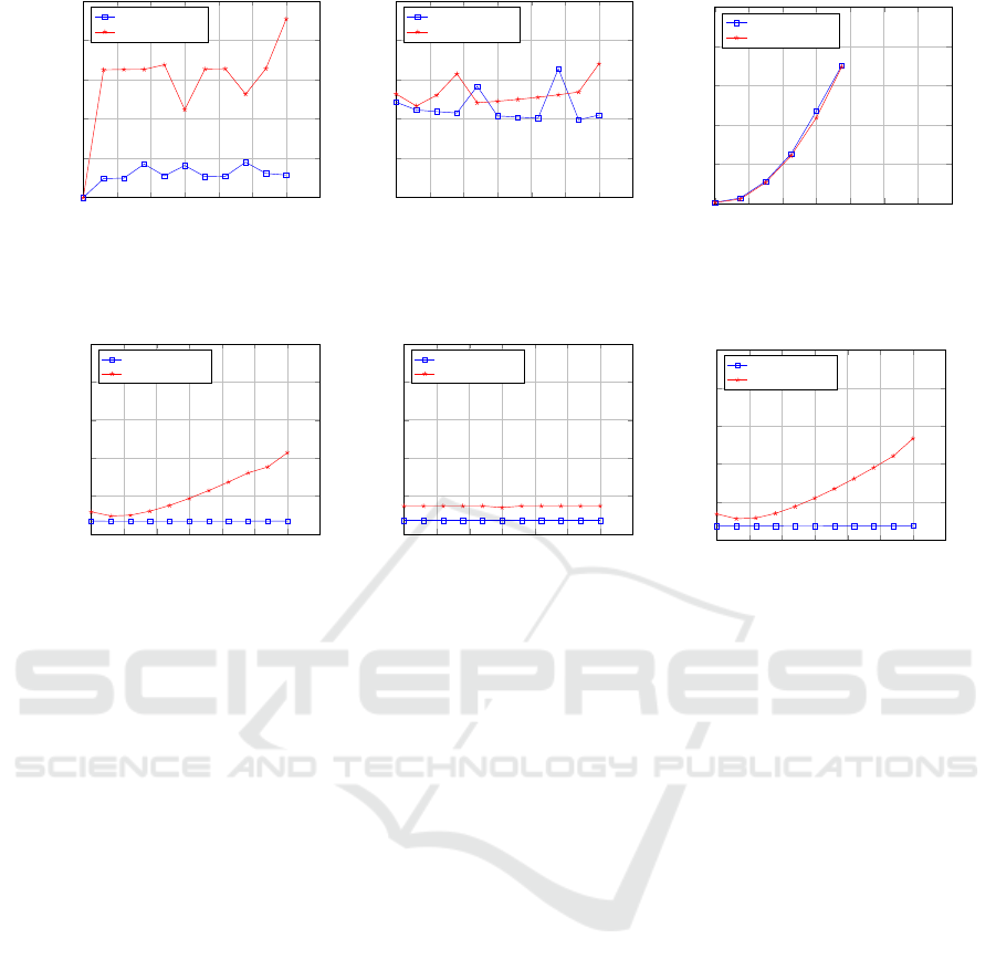
to its original orientation. The average displacement
error is proposed to evaluate the two methods:
err =
1
n
n
∑
i=1
u
original
i
− u
corrected
i
where n is the number of the feature points, u
original
i
is the original image coordinates of the point i, and
Visual Tilt Correction for Vehicle-mounted Cameras
867
0
5
10
15
20
25
30
0
1
2
3
4
5
Absolute pitch angle (Degree)
Displacement error (Pixels)
Forward motion
Sideways motion
(a)
0
5
10
15
20
25
30
0
1
2
3
4
5
Absolute roll angle (Degree)
Displacement error (Pixels)
Forward motion
Sideways motion
(b)
0 4 8 12
16
20 24
0
20
40
60
80
100
Absolute pitch and roll angles (Degree)
Displacement error (Pixels)
Forward motion
Sideways motion
(c)
Figure 2: The displacement error of the ground plane normal approach w.r.t the applied rotation, (a): pitch rotation is applied,
(b): roll rotation is applied, and (c): both pitch and roll rotations are applied.
0
5
10
15
20
25
30
0
0.5
1
1.5
2
2.5
Absolute pitch angle (Degree)
Displacement error (Pixels)
Forward motion
Sideways motion
(a)
0
5
10
15
20
25
30
0
0.5
1
1.5
2
2.5
Absolute roll angle (Degree)
Displacement error (Pixels)
Forward motion
Sideways motion
(b)
0
5
10
15
20
25
30
0
0.5
1
1.5
2
2.5
Pitch and roll angle (Degree)
Displacement error (Pixels)
Forward motion
Sideways motion
(c)
Figure 3: The displacement error of the vanishing points approach w.r.t the applied rotation, (a): pitch rotation is applied, (b):
roll rotation is applied, and (c): both pitch and roll rotations are applied.
u
corrected
i
is the image coordinates of the point i in the
corrected image using our approaches.
Fig. 2 shows the average displacement error in
pixels between the original and corrected image using
the ground plane normal approach with respect to the
rotation applied. The ground plane normal approach
returns the camera to its correct orientation with good
precision when only a pitch or a roll rotation is ap-
plied. It still returns good precision when both pitch
and roll rotations contaminate the camera orientation
with small angles < 5°.
Fig. 3 shows the displacement error of the vanish-
ing points method with respect to the rotation applied.
The vanishing points approach recovers the camera
to its correct orientation with very accurate precision
during the forward motion, it also works efficiently
during the sideways motion with error < 1.5 pixels.
3.2 Experiments with Real Data
Tilt correction on real data is evaluated qualitatively, a
set of interesting situations are chosen where the pla-
nar motion constraint is broken.
For evaluating the ground plane normal correction
method, three consecutive camera images are selected
in each interesting situation, the corresponding points
located on the ground plane are established manually
between the first and second images, and between the
the second and third images. Remark that the third
image is required for correcting the second one as the
correcting homographies are not the same for differ-
ent images. The correction matrices for the first and
second images are computed from first-second and
second-third pairs, respectively.
For each pair the correction matrix R
tc
is esti-
mated. The homography matrix for unnormalized co-
ordinates is H = KR
tc
K
−1
, where K is the intrinsic
camera parameters matrix. The homography matrix
H is used to transform the image and retrieve the cor-
rected camera image.
Figures 4, 5, 6 show the original and the cropped
corrected camera images using the ground plane nor-
mal approach for different situations.
Vanishing points method starts with establishing
the corresponding feature points between two consec-
utive camera images using SURF method (Bay et al.,
2006), RANSAC is used with 2 pixels threshold and
fixed 100 iterations to robustly estimate the rotation
matrix. Unnormalized homography matrix is calcu-
lated H = KR
tc
K
−1
, and the first image is corrected
accordingly.
Figures 7, 8, 9 show the original and corrected im-
age pairs for different situation. The corresponding
inlier points are visualized which represent the van-
ishing points.
VISAPP 2022 - 17th International Conference on Computer Vision Theory and Applications
868
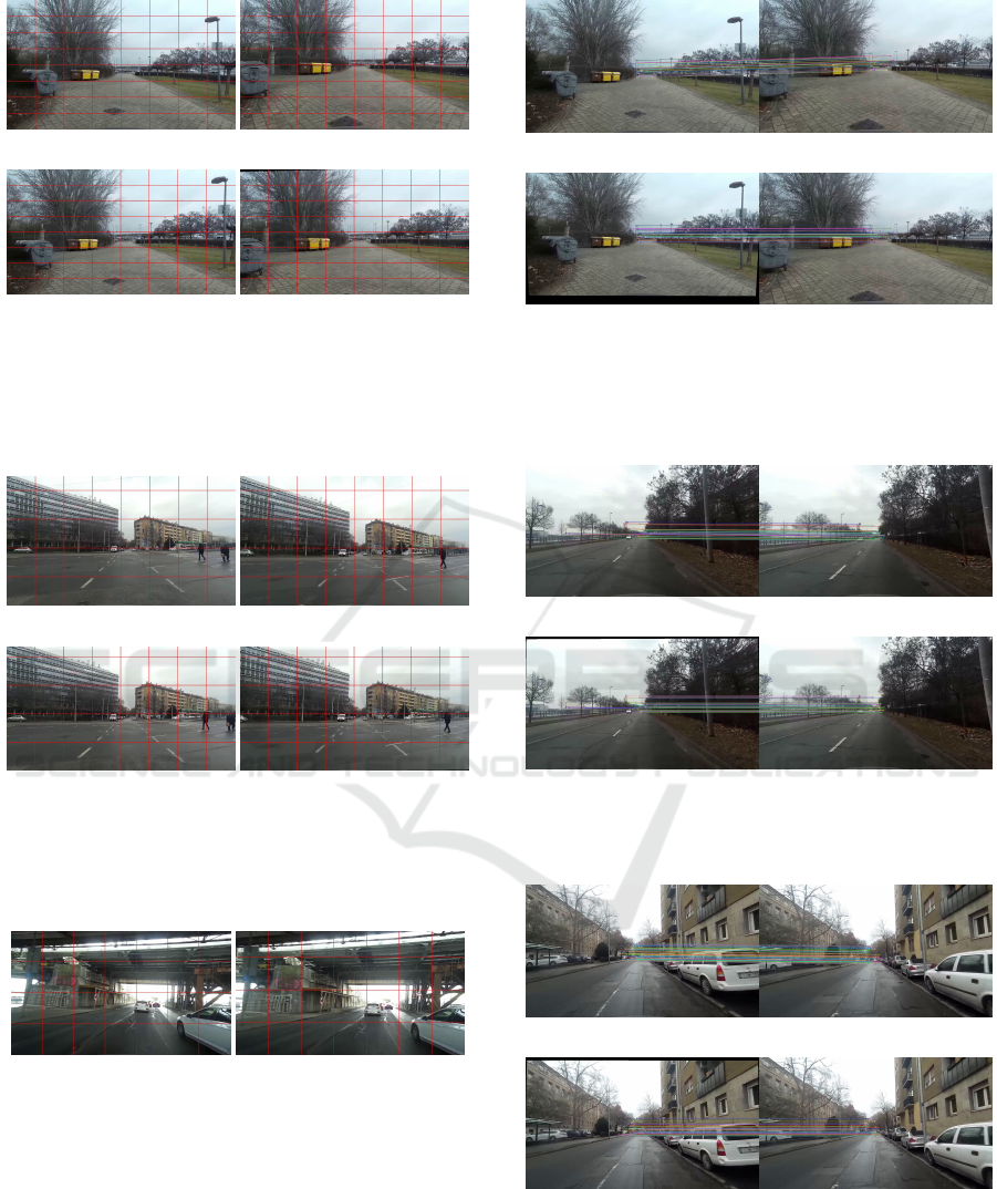
(a) First camera image. (b) Second camera image.
(c) Corrected first image. (d) Corrected second image.
Figure 4: Tilt correction using ground plane normal method,
the ground plane is non-flatten causing rotation about x-
axis. The two original images in the first row show the ver-
tical displacement caused by the non-flatten ground plane,
the second row shows how the displacement is corrected.
(a) First camera image. (b) Second camera image.
(c) Corrected first image. (d) Corrected second image.
Figure 5: Tilt correction using ground plane normal method,
the camera is shaking due to non-perfect camera mounting.
The first row shows the horizon line is displaced, the second
row shows the corrected camera images.
(a) Original camera image.
(b) Corrected camera image.
Figure 6: Tilt correction using ground plane normal method,
the car is turning right causing camera shaking. The hori-
zontal lines are sloped in the original image (a), the hori-
zontal lines are corrected in (b).
4 CONCLUSIONS AND FUTURE
WORK
We have addressed visual tilt correction for vehicle-
mounted cameras in this paper. For algorithms assum-
(a) Original camera image pair.
(b) Corrected image pair.
Figure 7: Tilt correction using vanishing points method
when ground plane is not-flatten causing rotation about x-
axis. The corresponding vanishing points are visualized in
the original and corrected pairs.
(a) Original camera image pair.
(b) Corrected image pair.
Figure 8: Tilt correction using vanishing points method, the
car moving with high speed causing shaking of the camera.
(a) Original camera image pair.
(b) Corrected image pair.
Figure 9: Tilt correction using vanishing points method,
camera shaking situation.
ing planar motion, it is essential that the image plane
should be perpendicular to the road surface. Two al-
gorithms have been proposed here. The first one ap-
Visual Tilt Correction for Vehicle-mounted Cameras
869

plies the ground plane as its normal coincides with the
gravity vector. The second algorithm filters the van-
ishing points close to the horizon and computes the
correction homography.
The accuracy of the algorithms are quantitatively
compared with the synthesized data. It is also demon-
strated that they are applicable for images of real
vehicle-mounted cameras.
Future Work. The proposed methods have been ap-
plied in this paper only for tilt correction. However,
the estimated vertical directions can be used for other
purposes. If the road is non-totally planar, it can be
detected. IMU sensors can measure the vertical di-
rection via gravity force, thus the proposed methods
can help in camera-IMU calibration. LiDAR-camera
calibration is also possible as the ground plane can be
estimated from LiDAR point clouds as well. These
are our research directions for the future.
ACKNOWLEDGEMENTS
Our work is supported by the project EFOP-3.6.3-
VEKOP-16-2017- 00001: Talent Management in Au-
tonomous Vehicle Control Technologies, by the Hun-
garian Government and co-financed by the Euro-
pean Social Fund. L. Hajder also thanks the sup-
port of the ”Application Domain Specific Highly
Reliable IT Solutions” project that has been im-
plemented with the support provided from the Na-
tional Research, Development and Innovation Fund
of Hungary, financed under the Thematic Excellence
Programme TKP2020-NKA-06 (National Challenges
Subprogramme) funding scheme.
REFERENCES
Arun, K. S., Huang, T. S., and Blostein, S. D. (1987). Least-
squares fitting of two 3-d point sets. IEEE Trans. Pat-
tern Anal. Mach. Intell., 9(5):698–700.
B. Triggs and P. McLauchlan and R. I. Hartley and
A. Fitzgibbon (2000). Bundle Adjustment – A Mod-
ern Synthesis. In Triggs, W., Zisserman, A., and
Szeliski, R., editors, Vision Algorithms: Theory and
Practice, LNCS, pages 298–375. Springer Verlag.
Bay, H., Tuytelaars, T., and Van Gool, L. (2006). Surf:
Speeded up robust features. In Leonardis, A., Bischof,
H., and Pinz, A., editors, Computer Vision – ECCV
2006, pages 404–417, Berlin, Heidelberg. Springer
Berlin Heidelberg.
Choi, S. and Kim, J.-H. (2018). Fast and reliable minimal
relative pose estimation under planar motion. Image
and Vision Computing, 69:103–112.
Fischler, M. A. and Bolles, R. C. (1981). Random sample
consensus: A paradigm for model fitting with appli-
cations to image analysis and automated cartography.
24(6):381–395.
Guan, B., Su, A., Li, Z., and Fraundorfer, F. (2019). Rota-
tional alignment of imu-camera systems with 1-point
RANSAC. In Pattern Recognition and Computer
Vision - Second Chinese Conference, PRCV 2019,
Xi’an, China, November 8-11, 2019, Proceedings,
Part III, pages 172–183.
Hajder, L. and Barath, D. (2020a). Least-squares optimal
relative planar motion for vehicle-mounted cameras.
In 2020 IEEE International Conference on Robotics
and Automation, ICRA 2020, Paris, France, May 31 -
August 31, 2020, pages 8644–8650.
Hajder, L. and Barath, D. (2020b). Relative planar mo-
tion for vehicle-mounted cameras from a single affine
correspondence. In 2020 IEEE International Confer-
ence on Robotics and Automation, ICRA 2020, Paris,
France, May 31 - August 31, 2020, pages 8651–8657.
Hartley, R. (1997). In defense of the eight-point algorithm.
IEEE Transactions on Pattern Analysis and Machine
Intelligence, 19(6):580–593.
Hartley, R. I. and Zisserman, A. (2003). Multiple View Ge-
ometry in Computer Vision. Cambridge University
Press.
Kukelova, Z., Bujnak, M., and Pajdla, T. (2008). Polyno-
mial eigenvalue solutions to the 5-pt and 6-pt relative
pose problems. In Proceedings of the British Machine
Vision Conference 2008, Leeds, UK, September 2008,
pages 1–10.
Li, H. and Hartley, R. I. (2006). Five-point motion estima-
tion made easy. In 18th International Conference on
Pattern Recognition (ICPR 2006), 20-24 August 2006,
Hong Kong, China, pages 630–633.
Malis, E. and Vargas, M. (2007). Deeper understanding of
the homography decomposition for vision-based con-
trol. PhD thesis, INRIA.
Nister, D. (2004). An efficient solution to the five-point
relative pose problem. IEEE Transactions on Pattern
Analysis and Machine Intelligence, 26(6):756–770.
Ortin, D. and Montiel, J. M. M. (2001). Indoor robot motion
based on monocular images. Robotica, 19(3):331–
342.
Saurer, O., Vasseur, P., Boutteau, R., Demonceaux, C.,
Pollefeys, M., and Fraundorfer, F. (2017). Homog-
raphy based egomotion estimation with a common
direction. IEEE Trans. Pattern Anal. Mach. Intell.,
39(2):327–341.
Stachniss, C., Leonard, J. J., and Thrun, S. (2016). Simul-
taneous localization and mapping. In Springer Hand-
book of Robotics, pages 1153–1176.
Weiss, S. and Siegwart, R. (2011). Real-time metric state
estimation for modular vision-inertial systems. In
IEEE International Conference on Robotics and Au-
tomation, ICRA 2011, Shanghai, China, 9-13 May
2011, pages 4531–4537.
VISAPP 2022 - 17th International Conference on Computer Vision Theory and Applications
870
