NEMA: 6-DoF Pose Estimation Dataset for Deep Learning

Philippe P

erez de San Roman

1,2

, Pascal Desbarats

, Jean-Philippe Domenger

and Axel Buendia

3,4

Univ. Bordeaux, CNRS, Bordeaux INP, LaBRI, UMR 5800, F-33400 Talence, France

ITECA, 264 Rue Fontchaudiere, 16000 Angoul

eme, France

CNAM-CEDRIC Paris, 292 Rue Saint Martin, 75 003 Paris, France

SpirOps, 8 Passage de la Bonne Graine, 75011, Paris, France

jean-philippe.domenger@u-bordeaux.fr, axel.buendia@cnam.fr

Keywords:

Deep Learning, 6-DOF Pose Estimation, 3D Detection, Dataset, RGB-D.

Abstract:

Maintenance is inevitable, time-consuming, expensive, and risky to production and maintenance operators.

Porting maintenance support applications to mixed reality (MR) headsets would ease operations. To function,

the application needs to anchor 3D graphics onto real objects, i.e. locate and track real-world objects in three

dimensions. This task is known in the computer vision community as Six Degree of Freedom Pose Estimation

(6-Dof) and is best solved using Convolutional Neural Networks (CNNs). Training them required numerous

examples, but acquiring real labeled images for 6-DoF pose estimation is a challenge on its own. In this article,

we propose ﬁrst a thorough review of existing non-synthetic datasets for 6-DoF pose estimations. This allows

identifying several reasons why synthetic training data has been favored over real training data. Nothing can

replace real images. We show next that it is possible to overcome the limitations faced by previous datasets by

presenting a new methodology for labeled images acquisition. And ﬁnally, we present a new dataset named

NEMA that allows deep learning methods to be trained without the need for synthetic data.

1 INTRODUCTION

Equipment used in manufacturing plants need main-

tenance. They include wearing parts that have to be

replaced periodically. They can also fail in which

case the cause must be diagnosed and actions must

be taken to repair them. Maintenance has increased

since production became more and more automated.

Guides are provided by Original Equipment Manufac-

turer (OEM) in order to ease maintenance and repairs.

These guides usually come in paper form, spanning

from a single sheet to several binders, or digital doc-

uments. These documents are unpractical for several

reasons: • Operators have to search for the solution to

their problems using index tables. • They have to un-

derstand the written actions and the drawn schemat-

ics explaining how to solve the problems. • Any in-

formation has to be pinpoint on the actual machine.

Thus operators waste time carefully going through

these documents, understanding them, and applying

the solution. If they don’t, they risk mistakes that

could cause more damage, wasted time, money or

worse might injure them. Moreover, adding feedback

and knowledge gained over time to those documents

means having to reprint them. That’s why software

solutions have been implemented to solve the above

mentioned issues. These softwares include a compre-

hensive 3D interactive view that helps understanding

and locating the problem and animations detailing the

actions and processes to solve the problem. They also

contain chats with co-workers, internal experts, OEM

support team and AI agents that help diagnose the

problem and highlight the best solutions. These soft-

wares can be expanded by the developers or the users

to include better diagnostics and solutions. But even

with such a software, operators have to switch from

working on the actual problem and application. Thus

some of the above mentioned challenges remain true.

They still have to be careful to correctly understand

instructions. Interaction with a laptop, tablette or

smartphone is as problematic as interacting with pa-

per documents while working. Especially with indi-

vidual protective equipment such as gloves and safety

glasses. With the release of the Microsoft Hololens 2

professionals have an ”on the shelf” solution to these

problems. The headset provides a heads up display

placed directly in the line of sight of the user. Holo-

grams can be displayed in three dimensions in the en-

682

Pérez de San Roman, P., Desbarats, P., Domenger, J. and Buendia, A.

NEMA: 6-DoF Pose Estimation Dataset for Deep Learning.

DOI: 10.5220/0010913200003124

In Proceedings of the 17th International Joint Conference on Computer Vision, Imaging and Computer Graphics Theory and Applications (VISIGRAPP 2022) - Volume 4: VISAPP, pages

682-690

ISBN: 978-989-758-555-5; ISSN: 2184-4321

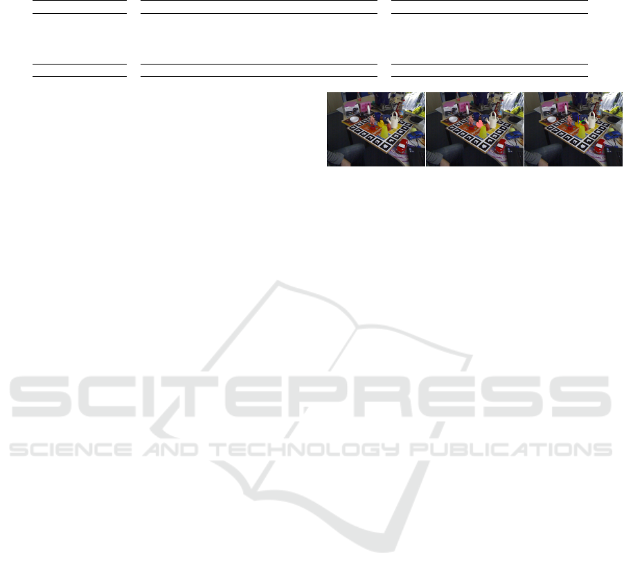
Table 1: Datasets comparison.

Dataset

Linemod

Occluded

T-Less (test)

YCB Video (test)

NEMA (ours)

(a) Depth errors.

µ(δ

) ± σ(δ

) µ(|δ

|) ± σ(|δ

|) Outliers

1.49 ± 07.75 mm 5.07 ± 6.05 mm 7.30 %

3.27 ± 07.52 mm 5.54 ± 6.05 mm 12.15 %

3.02 ± 12.15 mm 8.97 ± 8.74 mm 7.74 %

1.11 ± 05.09 mm 2.80 ± 4.39 mm 20.60 %

1.09 ± 03.05 mm 2.24 ± 2.61 mm 10.37 %

(b) Visibilities.

µ(v) ± σ(v) min(v) max(v)

96.47 ± 03.68 % 56.72 % 100 %

79.31 ± 24.23 % 0.05 % 100 %

83.06 ± 26.09 % 0 % 100 %

89.19 ± 15.65 % 7.54 % 100 %

62.72 ± 23.80 % 32.33 % 98.44 %

vironment without occulting what the user sees. An

eye tracker, gesture and voice recognition allow for

natural interactions with the visuals. But the software

can only work correctly if the 6-DoF pose estimation

module is reliable enough. This task, known as 6-

DoF pose estimation, is not a solved problem, particu-

larly when challenging factors such as occlusions and

changing lights come into play. Furthermore when

complex objects common in industrial equipment are

considered: textures less, metallic, transparent, sym-

metric or ambiguous. State of the art 6-DoF pose es-

timation methods are using CNNs. They require nu-

merous training examples consisting of an image, the

3D euler angles and the translation vector for each ob-

ject present in it (3+3 scalar values thus the name 6-

DoF). Models and camera intrinsic parameters must

be known by the application or estimated from the

images beforehand. Not many datasets provide re-

searchers and developers with such data. Recently

photorealistic render softwares made it possible to

train CNNs using synthetic images. The quality of

renderings allows to train networks that can then gen-

eralise to real situations in production. But validation

is also performed on real images to ensure robustness

of the results in real situations.

Summary

In this article we focus on the data rather than the

methods for 6-DoF pose estimation. In the ﬁrst sec-

tion, we study existing datasets, trying to identify

their limitations and what in the acquisition setup was

the cause. Next we propose our ﬁrst contribution

which is a new protocol to capture 6-DoF pose es-

timation datasets. This section includes details about

the hardware used and how to build it yourself. The

third and ﬁnal section presents the new dataset that we

recorded called NEMA-22 in comparison to previous

ones.

2 EXISTING DATASETS

Designing robust and economic networks for 6-DoF

pose estimation is key to enabling mixed reality ap-

plications to work. The ingenuity that goes into label

Figure 1: Sample image of the Linemod dataset.

expression, network architecture design, and training

procedures are tremendous. But it is even more chal-

lenging if the data needed for training and testing are

insufﬁcient or not reliable.

In this section, we review existing non-synthetic

datasets for 6-DoF pose estimation. We will present

these datasets, along with their setup and protocol.

Then we will look at the objects they chose and de-

tail image statistics to outline the challenges of these

datasets. We will look into any existing semantic gap

between training and test/validation in terms of ob-

ject visibility and object appearance. These can be

addressed using data augmentation to some extent.

Point of view (i.e., pose space) could also vary be-

tween training and testing images, which is difﬁcult to

bridge using image augmentation as the object’s ap-

pearance changes with them. And of course, we will

look at label quality as any outlier that contributes to

training can destabilize it. Our main objective is to

assert if these datasets are suited for 6 DoF pose es-

timation CNNs, identify what solution they offer to

speed acquisition of the data while preserving the ac-

curacy of the labels, and how we can improve upon

them.

2.1 Linemod

History and Information. Linemod was published

in 2012 by Stefan Hinterstoißer, Vincent Lepetit, Slo-

bodan Ilic, Stefan Holzer, Gary Bradski, Kurt Kono-

lige and Nassir Navab (Hinterstoisser et al., 2013). It

was recorded to illustrate and validate their work on

6-DoF pose estimation also called Linemod (Hinter-

stoisser et al., 2011). Data are available on Stefan

Hinterstoißer’s academic web page. Linemod is a col-

lection of 15 sequences of roughly 1200 images, one

for every object. In total the dataset contains 19 273

frames with the object in the center labeled. A sample

image is presented in ﬁgure 1.

NEMA: 6-DoF Pose Estimation Dataset for Deep Learning

683

Acquisition. The authors used a Kinect Gen 1 to

capture RGB and registered depth maps at 480p. One

object is placed at the center of a planar board covered

with calibration markers on its peripheral (Garrido-

Jurado et al., 2014). The markers are used to robustly

estimate the pose of the object. The recording was di-

vided into two steps: 1. To reconstruct the 3D model

of an object, it is placed alone on the board so that is it

completely visible. An untold number of pictures are

taken and using a voxel-based method, pixels are re-

projected to the model space. Finally, the voxels are

converted to points and re-meshed. 2. To record the

validation sequences other objects are added around

the labeled object to create occlusions. These are not

labeled and change location between frames or leave

the camera ﬁeld of view.

Statistics and Quality. The authors managed to ac-

quire evenly distributed points of view as we can see

in Figure 3b. This type of pose space is advanta-

geous because it can be split in training/test either

by selecting spaced-out points of view carefully, or

randomly, without impacting performances (Rad and

Lepetit, 2017). As for where the objects appear in

the image plane, there is a central bias as Figure 3a

shows. Moreover, all the foreground objects are in-

side the image boundaries.

To measure occlusions for their dataset, we com-

puted visibility by dividing the number of visible pix-

els by the number of pixels if the object was the

only one on-screen. The average visibility is 96.47 ±

3.68 %. Minimum is 56.72 % and the maximum is

100% thus objects are most visible. But because some

background objects can come in front of the fore-

ground object, and because they are not labeled, they

create occlusions that we could not take into account

in these statistics.

To evaluate the quality of the pose labels we com-

puted the mean pixel-to-pixel depth errors between

picture depth maps and depth maps rendered at the

ground truth pose as proposed by (Hoda

n et al., 2017).

Pixels for which the difference is greater than 50 mm

are attributed to depth sensor inaccuracies and are

not taken into account. The overall mean error is

1.49 mm and the mean absolute error is 5.07 mm with

7.3 % outliers. As we will see later compared to other

datasets this error is small thanks to calibration mark-

ers (see table 1).

About the reconstructed 3D models. The voxel-

based reconstruction method worked great for simple

objects (Ape, Duck, Cat) but others have holes or re-

meshing errors (Bowl, Cup, Lamp). This harms seg-

mentation labels quality that impacts the image pre-

processing pipeline. It also affects the error compu-

Figure 2: Sample image of the Occluded dataset.

tation by decreasing the number of considered pixels.

Moreover, texts such as the ”Bosh” logo on the driller

are not reconstructed at all. Furthermore, any renders

of these objects will have poor ﬁdelity.

Usage and Limitations. Linemod, the pose estima-

tion method, was based on templates computed using

renderings and only relies on 3D models for training.

Thus, the dataset was never intended for training, and

surely not for training a 6-DoF pose estimation deep

model. When repurposing it to such applications, one

is faced with several problems: • There are not enough

images / labeled instances. • The calibration markers

could bias training. • Unlabeled objects create un-

traceable occlusions. • Reconstructed 3D models are

of low quality.

To overcome these problems, two solutions have

been proposed: 1. It is possible to extract the fore-

ground of the object to get rid of calibration markers

and other objects, and use random backgrounds (Rad

and Lepetit, 2017; Xiang et al., 2017; Peng et al.,

2019; Tekin et al., 2017). But this process creates

highly unrealistic images where the object seems to

ﬂoat mid-air. Relations, scales, and perspectives are

completely false because background and foreground

are not pictured using the same camera nor at the

same pose. As mentioned, other unlabeled objects can

also ﬁnd their way into the foreground and destabilize

training. 2. It is also possible to use rendering to train

the model (Xiang et al., 2017; Hoda

n et al., 2020).

But as mentioned, the quality of the models makes it

difﬁcult to create photo-realistic images.

2.2 Linemod Occluded

History and Information. Two years after the re-

lease of Linemod, Eric Brachmann, Alexander Krull,

Frank Michel, Stefan Gumhold, Jamie Shotton, and

Carsten Rother contributed annotations for more ob-

jects visible in the ”Bench Vise Blue” sequence

(Brachmann et al., 2014). With the added labels the

dataset is known as ”Occluded”. Data are hosted on

the website of the Heidelberg university but a newer

version with veriﬁed labels is available as part of the

BOP benchmark. Figure 2 shows one image of this

sequence with the added labels.

VISAPP 2022 - 17th International Conference on Computer Vision Theory and Applications

684

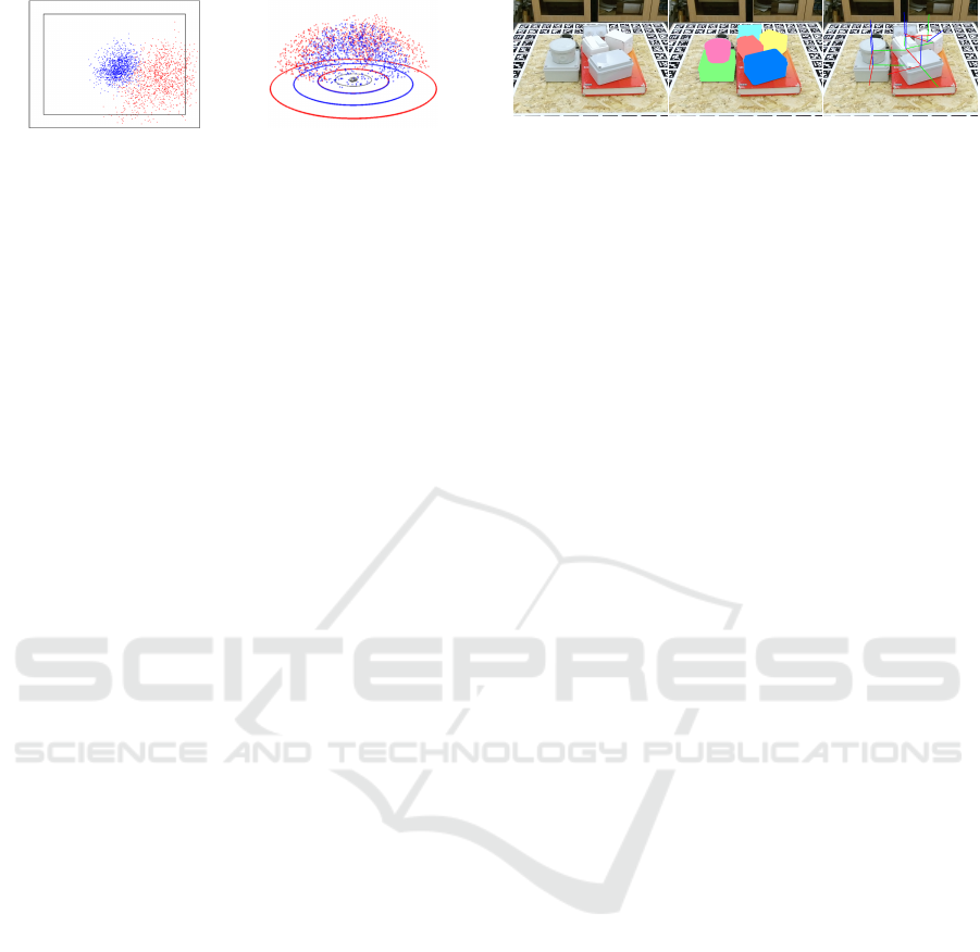
(a) (b)

Figure 3: Eggbox on-screen locations (a) and points of

views (b). Blue: Linemod, Red: Occluded.

Acquisition. Details for this dataset are found in the

supplementary materials of (Brachmann et al., 2014).

The process was semi-automatic. Ground truth la-

bels are deﬁned manually in the ﬁrst frame. Then the

transformation that moves from one frame to the next

following the camera motion is computed and applied

to the labels. If the pose of an object appears erro-

neous in one frame it is redeﬁned manually and the

process restarts. Finally, all poses are reﬁned using

the iterative closest point algorithm (Besl and McKay,

1992).

Statistics and Quality. The goal of the authors was

to get occlusions to benchmark against them. The

Duck is once occluded up to 99.95 % (0.05 % of vis-

ibility). Overall average visibility is 79.31 %, but

with a standard deviation of 24.23 %. Compared to

Linemod (96.47 ± 3.68 %) the objects are signiﬁ-

cantly more occluded. It is also worth mentioning that

the ”Egg Box” and ”Glue” ”objects are sometimes la-

beled but are outside of the camera ﬁeld of view. The

pose space of the added labels is similar in distribu-

tion to the one of Linemod as we can see in Figure

3b. But the distance to the objects can be greater. For

example, in Linemod, the ”Egg Box” is viewed at dis-

tances ranging from 0.67 m to 1.10 m. In Occluded it

is viewed at distances ranging from 0.66 m to 1.50 m.

So 1 cm closer and up to 40 cm further! With the oc-

cluded labels, the central image bias is gone as we can

see in Figure 3a. This is because some of the objects

are on the edge of the table. Thus, the camera does

not look at them and sometimes does not see them at

all. As we mentioned earlier, some objects were oc-

cluding the foreground objects of Linemod but there

were no labels. So, we had no idea these occlusions

were taking place. The labels of Occluded help with

this problem. If we look at the ”Bench Vise” the num-

ber of outliers is reduced from 7.51% to 6.50% while

the average absolute depth error remains close. This

proves that the added labels help identify and reduce

untraceable occlusions.

Usage and Limitations. Occluded build upon

Linemod by adding occlusions. By doing so its

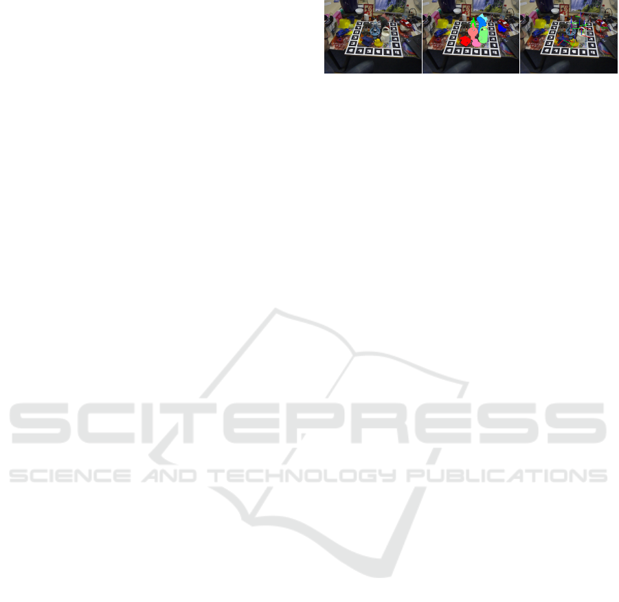
Figure 4: Sample image of the T-Less dataset.

authors solved the issues of untraceable occlusions

that affected the quality of labels. They also im-

proved upon the number of labeled instances. Finally,

they created a domain adaptation challenge between

the pose space of Linemod and Occluded. Just as

Linemod, this dataset is intended for template-based

methods that are trained using renders and is only in-

tended for testing. Thus, when training a deep model

for 6-DoF pose estimation 3 challenges remain, plus

the added challenges: 1. There are not enough images

/ labeled instances. 2. The calibration markers could

bias training. 3. Reconstructed 3D models are of low

quality. 4. There are extensive occlusions. 5. There

is a domain gap between Linemod / Occluded. Op-

tions to deal with these problems are the same as

for Linemod: 1. Use synthetic training images whose

quality is limited by the quality of the 3D models.

2. Use extensive image augmentation that end-up cre-

ating highly unrealistic images. Because training is

usually done on the Linemod images and testing on

the Occluded images. Augmentation must address

both the occlusions and the pose domain adaptation

challenges.

2.3 Texture Less (T-Less)

History and Information. T-LESS (Hoda

n et al.,

2017) was designed and pictured by Tom

s Hoda

Pavel Haluza,

an Obdr

alek, Ji

ı Matas, Manolis

Lourakis, et Xenophon Zabulis. The dataset focuses

on 30 industry-relevant challenging objects with no

distinct colors, shapes, or symmetries. The 30 train-

ing scenes have around 1 200 images and the test

scenes around 500. The dataset can be downloaded

on the ofﬁcial web page or as part of the BOP chal-

lenge.

Acquisition. Three cameras are used to acquire the

dataset: a Microsoft Kinect V2 (540p), a Prime-

sense Carmine 1.09 (540p) and a Canon Ixus 950 IS

(1920p). 3D CAD models are provided in STL for-

mat with a very detailed mesh but are not parametric

CAD models. The authors used a turntable that al-

lows them to quickly capture images at different an-

gles. It is covered on the top and sides with calibration

markers to accurately retrieve the pose of objects on

it. The camera mount allows them to adjust the cam-

NEMA: 6-DoF Pose Estimation Dataset for Deep Learning

685

(a) (b)

Figure 5: Object 01 on-screen locations (a) and points of

views (b). Blue: training, Red: test.

era height and tilt. The recording is divided into two

steps: 1. Training images feature a single object over

a black background at the center of the turntable. Im-

ages are cropped to have the object in the center and

to remove any visible markers. 2. Test images feature

multiple objects over various table tops. Multiple ob-

jects are placed, some of which are unlabeled (books,

bowls). Then the mesh of the whole scene is recon-

structed, the 3D models are aligned to it to compute

their pose. Finally, a manual inspection of the labels

is performed, and if needed they are corrected manu-

ally.

Statistics and Quality. The points of view are lo-

cated in a sphere as we can see in ﬁgure 5b. Like

in Linemod the object is located in the middle of the

training images and similarly to Occluded the test ob-

ject appears anywhere in the test images as we can see

in ﬁgure 5a. Objects are viewed from further away in

the test images. For instance, ”Object 01” is seen

at distance ranging from 0.62 m to 0.66 m in training

and at distance ranging from 0.64 m to 0.93m for test-

ing. Visibility is assured in the training images, but

in the test images, it averages 83.06 ± 26.09 % and

can be null for many objects. Authors of the T-Less

were the ﬁrst to evaluate the quality of the labels they

provided. They measured a 4.46mm average depth er-

ror. We measured 5.36mm for the training depth maps

and 3.02 mm for the test ones. The proportion of out-

liers that were excluded from computation is 5.46 %

for the training depth maps and 7.74 % for the test

ones. The use of a turntable with calibration mark-

ers, the solid camera rig, and the rigorous acquisition

protocol allowed the authors to create a dataset with

accurate labels.

Usage and Limitations. T-Less is intended for

methods that build templates and model distance to

the object as a scaling parameter. Thus, they do

not need training images at various distances, this is

why the training images are all shot at the same dis-

tance to the objects and feature a single object. The

test scenes are very different. They feature multiple

Figure 6: Sample image of the YCB Video dataset.

objects with occlusions. Thus, the pose space, dis-

tance to the objects, and on-screen location domains

are unlike. When training deep network for 6-DoF

pose estimation on T-Less the following challenges

apply: 1. There are not enough images / labeled in-

stances. 2. Objects are difﬁcult (textureless, symmet-

ric). 3. Training images have a black background.

4. Large domain gap between training/test. Such dif-

ﬁculties are hard to overcome for deep models. Im-

age augmentation can solve some of them as exper-

iments on Linemod Occluded have proven (Rad and

Lepetit, 2017). Again, the resulting images are far

from realistic. But the added challenge of object ap-

pearance is difﬁcult with these few images. This is

why deep models have struggled to solve T-Less using

only real images. The only viable solution on T-Less

is to use synthetic images for training (Pitteri et al.,

2019; Hoda

n et al., 2020). The high-quality 3D mod-

els are well suited to create photo-realistic renders.

2.4 YCB Video

History and Information. Also in 2017, the YCB

Video was designed by Xiang Yu, Schmidt Tan-

ner, Narayanan Venkatraman, and Fox Dieter (Xiang

et al., 2017). It is the ﬁrst dataset designed to accom-

modate the training and testing of 6-DoF pose estima-

tion deep networks. YCB Video can be downloaded

from the Pose CNN website but we used the BOP

challenge repository. It pictures 21 objects of the

YCB objects (Calli et al., 2017). Some objects have

challenging textureless appearances, other are identi-

cal to a scaling factor. Scale is ambiguous in 6-DoF

pose estimation that assumes rigid objects at constant

scale. They recorded 92 videos provided with pose

labels. In total the dataset contains 133 827 labeled

frames with aligned depth maps at 480p. A sample

im- age is displayed in Figure 6.

Acquisition. Authors wanted to avoid as much as

possible manual annotations which are a source for

errors, especially because labeling 3D poses is very

tricky from 2D images. They also wanted as many

images as possible to train a deep model. That is why

they decided to ﬁlm scenes to obtain 30 images per

second. The pose of each object is aligned in the ﬁrst

frame using a signed distance function (Osher and

Fedkiw, 2003): rendered depth is aligned to the depth

VISAPP 2022 - 17th International Conference on Computer Vision Theory and Applications

686

(a) (b)

Figure 7: Coffee Can on-screen locations (a) and points of

views (b). Blue: training, Red: test.

frame. When moving to the next frame the camera

motion is computed and propagated to the pose labels.

Statistics and Quality. Because the recording pro-

cess is so different from previous datasets, the pose

space is also unlike previous ones. The points of view

of the Coffee Can are displayed in ﬁgure 7b. Poses

are no longer evenly distributed but are rather densely

sampled along the path of the camera. The locations

where objects appear on-screen follow the same pat-

tern as we can see in ﬁgure 7a. There is no central bias

and many objects end up outside the image bound-

aries. Visibility ranges from 0% to 100% with an av-

erage of 86.17 ± 19.84 % in the training images. And

it ranges from 7.54 % to 100 % in the testing images

with an average of 89.19 ± 15.65 %. So the dataset

includes signiﬁcant occlusions that are showcased in

the training images. The method used to annotate im-

ages automatically optimizes depth error in the depth

maps. So naturally, when we measure the error, it is

low: 1.11 ± 5.09 mm on average and 2.80 ± 4.39 mm

absolute average. But this optimization seems to have

failed on some images because we found 20.6 % of

outliers which is larger than other datasets (see table

1) and cannot be attributed only to depth sensor er-

rors.

Usage and Limitations. Because poses are not

sampled sparsely, the test sample cannot be selected

at random. Instead, some videos are used for training,

and others as test sequences. There are no calibra-

tion markers in the images so there is no need to erase

them. Because of how the dataset is recorded test-

ing points of view are far from the training ones. The

method described by the authors was able to general-

ize, achieving 75.9 % of accuracy. But later works

have shown that renderings that cover the ”miss-

ing” training poses helped better the result (Trem-

blay et al., 2018; Hoda

n et al., 2020). Not relying on

calibration markers makes it possible to record video

thus speeding up acquisition. But the measured out-

liers proportion indicates that it comes at the cost of

label quality in some frames. The quality of the la-

bels has already been criticized by its authors (Xiang

et al., 2017) and by the authors of the BOP challenge

(Hoda

n et al., 2020).

Critics

6-DoF pose estimation is a challenging task and

datasets should not contribute to more difﬁculties.

CNNs require more images to be trained compared

to template based methods. The only dataset in this

ﬁeld providing a sufﬁcient number of images is the

latest YCB Video dataset. But it contains images

with erroneous labels due to its recording and anno-

tation process. Older datasets, with better quality la-

bels, were meant for methods that used renderings of

the 3D models to build templates. Thus, they do not

contain the required number of images to train deep

CNN models. The images were not meant to be used

as training samples and contain visible markers that

must be erased to prevent biased results. But the rere-

sulting images are far from realistic. Because of these

reasons, the go-to solution is to use renders. While

their quality has improved, they have become cheap to

compute thanks to GPU and cheap to store thanks to

large hard drives and cloud storage. But can we trust

a deep CNN only trained on synthetic data in real-life

applications ? We believe a new dataset could learn

from the protocols of the existing ones and improve

upon their limitations.

3 NEMA-22 DATASET

In this section we present our new dataset called

NEMA. First we detail the hardware we chose and

why. Second we explain the protocol we followed to

record the dataset. Finally we showcase some images

and qualitive results of NEMA.

3.1 Hardware

To make a 6-DoF pose estimation any RGB-D camera

can work but they do not all offer the same quality and

ease of use. The objects considered need to provide

sufﬁcient challenges in order to objectively evaluate

network performances. The table setup and other ac-

cessories will also greatly impact the protocol for la-

bel acquisition. In general hardware impacts the time

spent to record the dataset and the label quality.

This subsection details the motivation and con-

straints that guided our hardware choices.

Camera. Microsoft Azure ($400) were not avail-

able at the time of the dataset recording. So we de-

cided to use the Intel Realsense d435i ($329). It’s

NEMA: 6-DoF Pose Estimation Dataset for Deep Learning

687

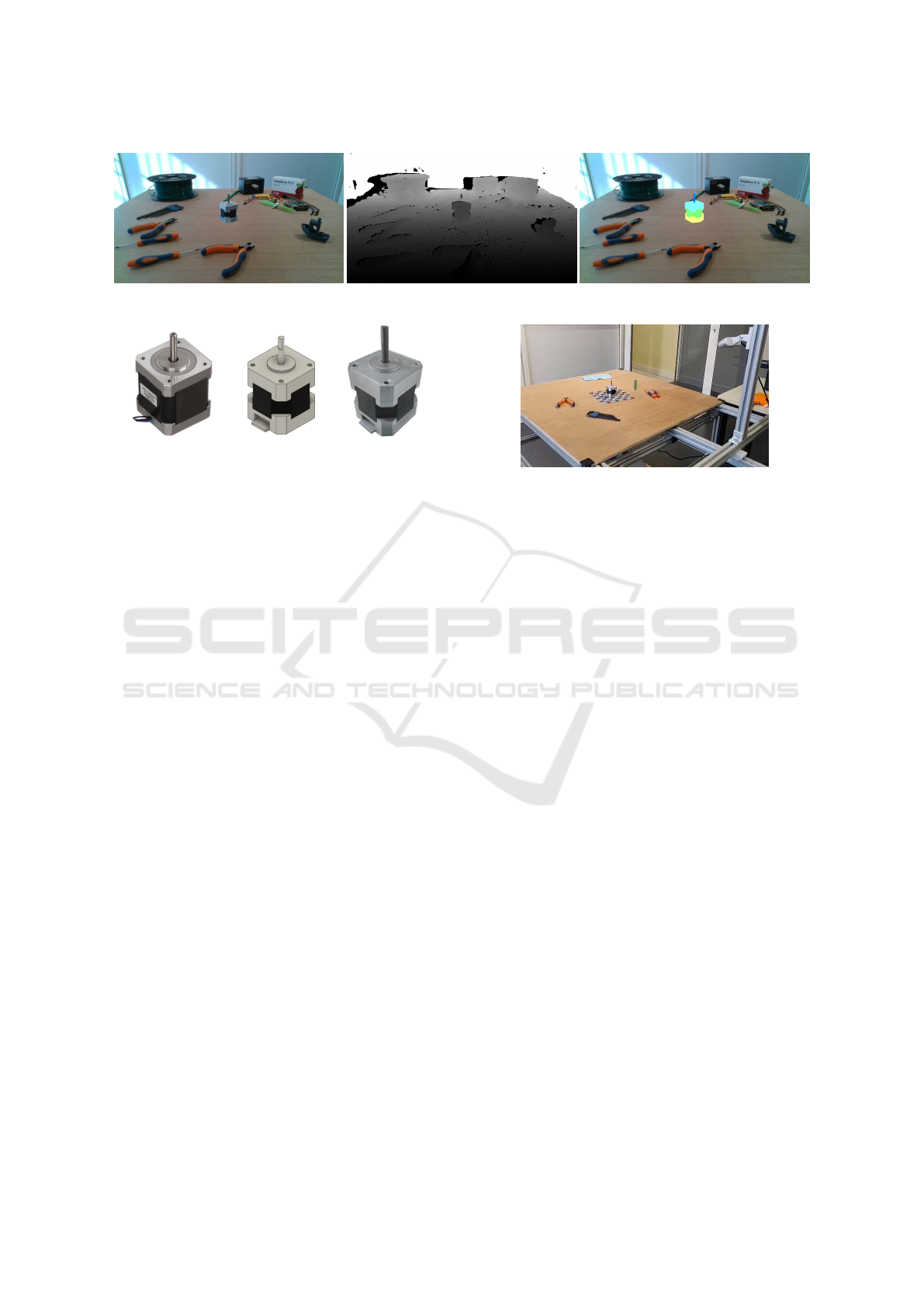
Figure 8: Sample image of our NEMA dataset with segmentation and pose labels.

Figure 9: NEMA 17 motor used in our dataset. Left: real,

middle: 3D design, right, 3D printed.

equipped with a Full HD camera and two infrared

cameras with HD capabilities. We conﬁgured the

camera to deliver registered color images and depth-

maps at 720p using Intel’s Realsense Python SDK

(free). Our dataset consists of pictures, not vid

eos.

Objects. For the objects we had several constraints

in mind. • We wanted parametric CAD models that

allow for low-poly exports of meshes and parametric

loss expression. • We wanted an object composed of

several pieces that can be assembled together. • We

wanted our object to look like industrial ones: texture

less, metallic and symmetric. • Moreover we wanted

anyone to have access to our object, free of charge.

To prototype this we designed a simpliﬁed repre-

sentation of a NEMA 17 stepper motor. We only in-

cluded the outer parts: bottom, body, top and shaft.

Nonetheless, we sized our pieces to be accurate to

the NEMA ICS 16-2001 (Association, 2001). All the

drawings were done in Fusion 360 then 3D printed on

un Ultimaker 2+. Figure 9 presents a real NEMA 17,

our design and the printed result.

This way we end up with an object composed of

four pieces, with challenging appearance and shape

for which we have precise and parametric 3D CAD

models. We make this design freely available with

printing settings so people can 3D print them and re-

produce our results.

Turn Table. After studying the existing datasets we

found a board with calibration markers is the most re-

liable solution to acquire pose labels. Combined with

a turning table it becomes rapid to acquire a full 360

◦

Figure 10: Table with the camera and a sample scene setup.

or more set of pictures. We only have to take back-

ground pictures to mask the markers.

On-shelf turn-tables are expensive, do not include

markers, and are thick. Any height added by the turn-

table will give the impression in the masked image

that the objects are ﬂoating mid air. We also need to

swap in and out the turntable to picture background

images.

So we imagined a simple turntable that we could

also 3D print. The top of the board is the only thing

above the table and it’s as thin as paper. A stepper

motor (28BYJ-48) placed under the table rotates the

top and micro-switch enables homing to 0

◦

. We used

an Arduino Nano Every over serial USB to control the

board using Python programming. The 3D models for

the board, motor casing, the Arduino ﬁrmware sketch

and the python serial communication software are all

made available for free.

Table and Supports. The table has a plywood top.

Its legs and the camera support are made with mod-

ular aluminum tubing and a few homemade parts. It

gives us plenty of room to accommodate the scenes

with background objects. The plans, parts list, and

custom parts designs are made available for free.

3.2 Protocol

We chose to use markers to obtain accurate pose la-

bels. If background images are not recorded using the

same camera and point of view then the perspective

in the image will be incorrect. Thus we decided to

record them using the same camera at the same loca-

tion. Our protocol allows us to position the camera,

VISAPP 2022 - 17th International Conference on Computer Vision Theory and Applications

688

then record the background, and ﬁnally automatically

record a 360

◦

rotation of the turn-table. The steps are

detailed below.

Setup Camera. We record color images and

aligned depth maps at a resolution of 1280×720 pix-

els. We set the frame rate to the default 30 FPS but

we do not rely on it.

Setup ChArUco. We used an 8×8ChArUco board.

The cell size is set to 24 mm which is half the width

of the bottom of our object. This trick allows us to

precisely align the object with the center of the board.

We provide a scaled PDF with the ChArUco board

ready to print in the dataset.

Setup Scene. The dataset can contain many scene.

Sequences of a scene will display the same objects

with the same positions and orientation with respect

to the ChArUco board. When creating a new scene

our software allows us to preview the pose labels on

the video stream. Each object is added by providing

its 3D model. Then their pose can be manually set

using translation and Euler angles. Other unlabeled

objects can be added in the background but they must

not occlude the ChArUco board or the labeled objects

on it. The turn-table can be rotated freely to ensure

correct pose labels.

Setup Sequence. A sequence contains all the pic-

tures acquired by the camera at a given point of view.

This includes the pictures acquired when rotating the

turn-table and the background. When creating a se-

quence we ﬁrst move the camera on its rig. We used

a measuring tape to move the camera 1 cm at a step

horizontally or vertically. We always tilt the camera

so that it looks at the center of the ChArUco board to

ensure central bias.

Background Image Acquisition. Once the camera

is placed we remove the foreground objects and the

ChArUco board and take the background picture.

Foreground Images Acquisition. We place back

the ChArUco board on the table and add back the

foreground objects. The same display as for the scene

setup allows us to realign precisely the pieces on the

board. Then we can set the rotation step between

two pictures to 0.5

◦

and hit record. The turn-table

will home iteself and start rotating. At each step a

foreground picture is taken, the pose of the ChArUco

board is estimated, the pose of the foreground objects

is computed and saved.

If for any reason the pose of the ChArUco board

cannot be estimated the recording stops. This is usu-

ally because the camera is too far out and markers can

not be detected. In that case we simply delete the se-

quence and move to the next one.

3.3 Statistics and Quality

Using the selected hardware and protocol we com-

pleted the recording of a complete scene composed

of 240 sequences. As we selected a step of 0.5

◦

for

the turntable each sequence is 720 images rich. This

brings the wall scene to 172 800 images. And in each

image 4 objects plus the charuco board are labeled.

This means that so far we have recorded 691 200 la-

beled object instances.

The points of views of each object are displayed in

ﬁgure 11. Just like in Linemod and TLESS we man-

aged to acquire evenly distributed points of views.

They can be split into a training and test set randomly.

Objects are occluded 62.72 % in average and 32.33 %

at most, which is reasonably low. We achieved central

bias as we can see in ﬁgure 12 and no object is out-

side the camera ﬁeld of view. Visibility is presented in

Table 2. It ranges from 32.33% to 98.44% with an av-

erage of 62.72 ± 23.80%. Individual objects have rel-

atively constant visibility as the scene layout does not

change (their standard deviations are all lower than

5 %).

We not only computed the depth error on the fore-

ground objects but also on the ChArUco board. The

quality of the labels is better than the previous dataset

as we can see in table 1. The average depth error is

1.089 ± 3.048 mm and absolute average depth error

is 2.235 ± 2.606 mm. Most of the outliers are con-

tributed by the shaft: 30.078 % of outliers. This is

also visible in the sample depth map (ﬁgure 8). This

very thin gray object is not pictured by the depth sen-

sor. The bottom, body and ChArUco have very little

outliers (∼ 4 %) and depth error (∼ 3 mm).

4 CONCLUSION

In this article we ﬁrst reviewed the existing datasets

for 6-DoF pose estimation. This review convinced us

that there is room for improvement. First the depth

cameras have improved both in terms of resolution

and image quality. Deep CNNs, especially full con-

volutional, can take advantage of larger image res-

olution. Second existing dataset either do not offer

enough images, or contain erroneous labels. This is

due to the protocol that was either not intended for

NEMA: 6-DoF Pose Estimation Dataset for Deep Learning

689

Table 2: NEMA-22 statistics.

Object(s)

Body

Bottom

Shaft

Top

Charuco

All

(a) Visibility.

min(v) max(v) µ(v) ± σ(v)

35.20% 60.76% 46.76 ± 04.35 %

35.26% 61.51% 48.33 ± 04.33 %

32.18% 41.19% 36.67 ± 01.09 %

95.38% 98.44% 96.77 ± 00.46 %

81.84% 87.87% 84.78 ± 01.36 %

32.33% 98.44% 62.72 ± 23.80 %

(a) Depth error.

µ(δ

) ± σ(δ

) µ(|δ

|) ± σ(|δ

|) Outliers

−2.275 ± 3.676 mm 3.108 ± 6.165 3.834 %

−0.671 ± 4.803 mm 2.686 ± 5.251 3.664 %

0.819 ± 1.836 mm 1.527 ± 1.487 30.078 %

1.143 ± 4.162 mm 3.163 ± 3.564 11.652 %

1.369 ± 2.595 mm 2.078 ± 2.189 2.628 %

1.089 ± 3.048 mm 2.235 ± 2.606 10.371 %

(a) Bottom (b) Body (c) Top (d) Shaft

Figure 11: NEMA on-screen locations.

(a) Bottom (b) Body (c) Top (d) Shaft

Figure 12: NEMA points of views.

deep models, or that relied on global optimization to

save time that can fail for some images.

Our protocol factories the manual steps and allow

for fast and robust image + label semi-automatic ac-

quisition. It can be applied to any camera. Other hard-

ware pieces are mostly 3D printed. We make the 3D

CAD models, printing settings, software to record the

dataset and the complete dataset available to anyone

for free. We hope people will contribute to the dataset

our create their own using our tools and protocol.

REFERENCES

Association, N. E. M. (2001). Nema ics 16, industrial

control and systems, motion/position, control motors,

controls and feedback devices. Standard, National

Electrical Manufacturers Association, 1300 N. 17th

street, Rosslyn, Virginia 22209.

Besl, P. and McKay, N. D. (1992). A method for registration

of 3-d shapes. IEEE Transactions on Pattern Analysis

and Machine Intelligence, 14(2):239–256.

Brachmann, E., Krull, A., Michel, F., Gumhold, S., Shotton,

J., and Rother, C. (2014). Learning 6d object pose es-

timation using 3d object coordinates. In Fleet, D., Pa-

jdla, T., Schiele, B., and Tuytelaars, T., editors, Com-

puter Vision – ECCV 2014, pages 536–551, Cham.

Springer International Publishing.

Calli, B., Singh, A., Bruce, J., Walsman, A., Konolige, K.,

Srinivasa, S., Abbeel, P., and Dollar, A. M. (2017).

Yale-cmu-berkeley dataset for robotic manipulation

research. The International Journal of Robotics Re-

search, 36(3):261–268.

Garrido-Jurado, S., Mu

noz-Salinas, R., Madrid-Cuevas,

F. J., and Mar

ın-Jim

enez, M. J. (2014). Auto-

matic generation and detection of highly reliable ﬁdu-

cial markers under occlusion. Pattern Recognition,

47(6):2280–2292.

Hinterstoisser, S., Holzer, S., Cagniart, C., Ilic, S., Kono-

lige, K., Navab, N., and Lepetit, V. (2011). Multi-

modal templates for real-time detection of texture-less

objects in heavily cluttered scenes. pages 858–865.

Hinterstoisser, S., Lepetit, V., Ilic, S., Holzer, S., Bradski,

G., Konolige, K., and Navab, N. (2013). Model based

training, detection and pose estimation of texture-less

3d objects in heavily cluttered scenes. In Lee, K. M.,

Matsushita, Y., Rehg, J. M., and Hu, Z., editors, Com-

puter Vision – ACCV 2012, pages 548–562, Berlin,

Heidelberg. Springer Berlin Heidelberg.

Hoda

n, T., Haluza, P., Obdr

alek,

S., Matas, J., Lourakis,

M., and Zabulis, X. (2017). T-LESS: An RGB-D

dataset for 6D pose estimation of texture-less objects.

IEEE Winter Conference on Applications of Computer

Vision (WACV).

Hoda

n, T., Sundermeyer, M., Drost, B., Labb

e, Y., Brach-

mann, E., Michel, F., Rother, C., and Matas, J. (2020).

BOP challenge 2020 on 6D object localization. Euro-

pean Conference on Computer Vision Workshops (EC-

CVW).

Osher, S. and Fedkiw, R. (2003). Signed Distance Func-

tions, pages 17–22. Springer New York, New York,

NY.

Peng, S., Liu, Y., Huang, Q., Zhou, X., and Bao, H. (2019).

Pvnet: Pixel-wise voting network for 6dof pose esti-

mation. In CVPR.

Pitteri, G., Ramamonjisoa, M., Ilic, S., and Lepetit, V.

(2019). On object symmetries and 6d pose estimation

from images. International Conference on 3D Vision.

Rad, M. and Lepetit, V. (2017). BB8: A scalable, accurate,

robust to partial occlusion method for predicting the

3d poses of challenging objects without using depth.

CoRR, abs/1703.10896.

Tekin, B., Sinha, S. N., and Fua, P. (2017). Real-time

seamless single shot 6d object pose prediction. CoRR,

abs/1711.08848.

Tremblay, J., To, T., and Birchﬁeld, S. (2018). Falling

things: A synthetic dataset for 3d object detection and

pose estimation. CoRR, abs/1804.06534.

Xiang, Y., Schmidt, T., Narayanan, V., and Fox, D. (2017).

Posecnn: A convolutional neural network for 6d

object pose estimation in cluttered scenes. CoRR,

abs/1711.00199.

VISAPP 2022 - 17th International Conference on Computer Vision Theory and Applications

690