Deep Depth Completion of Low-cost Sensor Indoor RGB-D using

Euclidean Distance-based Weighted Loss and Edge-aware Reﬁnement

Augusto R. Castro

1 a

, Valdir Grassi Jr.

1 b

and Moacir A. Ponti

2 c

Department of Electrical and Computer Engineering, S

ao Carlos School of Engineering, University of S

ao Paulo,

ao Carlos, Brazil

Instituto de Ci

encias Matem

aticas e de Computac¸

ao, Universidade de S

ao Paulo, S

ao Carlos, Brazil

Keywords:

Deep Learning, Depth Completion, RGB+Depth, Depth Sensing, Distance Transforms.

Abstract:

Low-cost depth-sensing devices can provide real-time depth maps to many applications, such as robotics and

augmented reality. However, due to physical limitations in the acquisition process, the depth map obtained

can present missing areas corresponding to irregular, transparent, or reﬂective surfaces. Therefore, when there

is more computing power than just the embedded processor in low-cost depth sensors, models developed to

complete depth maps can boost the system’s performance. To exploit the generalization capability of deep

learning models, we propose a method composed of a U-Net followed by a reﬁnement module to complete

depth maps provided by Microsoft Kinect. We applied the Euclidean distance transform in the loss function to

increase the inﬂuence of missing pixels when adjusting our network ﬁlters and reduce blur in predictions. We

outperform state-of-the-art methods for completed depth maps in a benchmark dataset. Our novel loss function

combining the distance transform, gradient and structural similarity measure presents promising results in

guiding the model to reduce unnecessary blurring of ﬁnal depth maps predicted by a convolutional network.

1 INTRODUCTION

Light Detection And Ranging sensors (LiDAR),

stereo cameras, and time-of-ﬂight sensor-based sys-

tems (like Microsoft Kinect) are technologies that en-

able depth measurement. The combination of depth

information captured by those resources and RGB im-

ages is commonly used in visual odometry, skeleton

tracking, path planning, and object 3D reconstruction.

The referred Microsoft Kinect sensor and the Intel

RealSense cameras can provide RGB and depth in-

formation (so-called RGB-D) at a high frame rate for

a low cost (Xian et al., 2020; Senushkin et al., 2020;

Atapour-Abarghouei and Breckon, 2018) and became

popular for depth acquisition as they allowed applica-

tions of 3D data in tasks where only 2D cameras were

previously applied.

However, the depth information provided by low-

cost real-time sensors usually presents missing data

in the form of holes caused by absent measures in

reﬂective, transparent, or irregular surfaces (Bapat

et al., 2015; Zhang and Funkhouser, 2018; Xian et al.,

https://orcid.org/0000-0002-4227-307X

https://orcid.org/0000-0001-6753-139X

https://orcid.org/0000-0003-2059-9463

2020; Huang et al., 2019; Atapour-Abarghouei and

Breckon, 2018). Also, those devices have a restricted

range that only allows measuring depth information

within an interval of minimum and maximum dis-

tances and often present noisy estimates for larger dis-

tances. As many applications have more computing

power than just the sensor processor, it is natural to

use methods to enhance the depth map by ﬁlling the

missing data and sharpening measures based on the

RGB data to boost the ﬁnal system results.

However, depth prediction and completing can be

addressed in different ways and may be referred to as

Single Image Depth Estimation, LiDAR Depth Com-

pletion, or Image Inpainting. In Single Image Depth

Estimation, the aim is to produce accurate depth maps

from RGB images. Recent studies applied geometric

cues provided by sparse and noisy LiDAR data, se-

mantic segmentation, or surface normal vectors to im-

prove the ﬁnal depth prediction (de Queiroz Mendes

et al., 2021; Qi et al., 2020), however the main focus

still relies on the RGB input. Nevertheless, the ability

to infer depth from RGB data may help to ﬁll large

missing areas.

LiDAR-oriented methods rely on semi-dense

depth maps obtained by uniformly sampling a

204

Castro, A., Grassi Jr., V. and Ponti, M.

Deep Depth Completion of Low-cost Sensor Indoor RGB-D using Euclidean Distance-based Weighted Loss and Edge-aware Reﬁnement.

DOI: 10.5220/0010915300003124

In Proceedings of the 17th International Joint Conference on Computer Vision, Imaging and Computer Graphics Theory and Applications (VISIGRAPP 2022) - Volume 4: VISAPP, pages

204-212

ISBN: 978-989-758-555-5; ISSN: 2184-4321

ﬁlled depth map completed using interpolation

methods and ﬁltering (Senushkin et al., 2020;

de Queiroz Mendes et al., 2021). When compared to

semi-dense depth maps provided by Kinect sensors,

depth maps obtained by uniformly sampling LiDAR

interpolation measurements do not present the same

kind of missing areas observed in our work. The uni-

formly sampling step may reproduce the same density

of valid pixels but fails in concentrating them on ob-

ject edges or reﬂective, transparent, or irregular sur-

faces (Senushkin et al., 2020). Furthermore, while

outside environments are the ordinary case of LiDAR

sensors application, low-cost depth sensing devices

are preferred for indoor tasks.

Finally, image inpainting consists of methods for

repairing missing areas in an image, usually tackling

small and thin regions or large ﬂat areas (Xian et al.,

2020). The focus is obtaining feasible results based

on the scene rather than generating accurate pixel val-

ues, as required by depth completion (Huang et al.,

2019). Nevertheless, (Huang et al., 2019) used an im-

age inpainting method for depth completion using a

self-attention mechanism and gated convolutions.

In this paper, we assume the input is a RGB-D

image provided by a low-cost sensor for an indoor

scene containing missing regions, while the output

is the complete depth map of the view. Our method

aims to ﬁll in all missing areas in the depth map using

cues provided by the full RGB image. Therefore, the

ground truth depth maps provided by the dataset must

be composed of fully completed depth maps. LiDAR

data would not be appropriate in our context since

the scale difference might not provide the same spa-

tial distribution of holes. For example, while miss-

ing areas across object edges reduce as the distance

to the sensor increases, outdoor scenes may present

large holes at the top of the depth map correspond-

ing to the sky. We investigate the use of an Encoder-

Decoder Convolutional Neural Network (CNN) using

a novel loss function that combines the depth estima-

tion with an inverted Euclidean Distance Transform

(EDT). Our contribution is to show the EDT can guide

the training to better complete large missing regions

that represent the most difﬁcult part of such a prob-

lem, and to enhance it with a edge-aware reﬁnement

module for smaller error rates.

The proposed method has two modules: a depth

completion step from RGB-D input and a reﬁnement

module using GeoNet++ (Qi et al., 2020) to enhance

the full depth obtained from the depth completion

module. Figure 1 provides an overview of both mod-

ules and shows where the RGB image is used to guide

the depth completion of a raw depth map.

1.1 Related Works

Although previous studies on depth map completion

have addressed the task using traditional image pro-

cessing techniques, such as bilateral ﬁltering (Chen

et al., 2012; Bapat et al., 2015) and Fourier trans-

form (Raviya et al., 2019), deep neural networks can

be particularly useful to learn from existing data in

an attempt to generalize to unseen maps (Ponti et al.,

2021).

In terms of deep learning-based depth comple-

tion of semi-dense indoor depth maps, the method

described by (Zhang and Funkhouser, 2018) was the

ﬁrst to deﬁne the problem of ﬁlling large missing ar-

eas in depth maps acquired using commodity-grade

depth cameras. The solution presented predicts local

properties of the visible surface at each pixel (occlu-

sion boundaries and surface normals) and then apply a

global optimization step to solve them back to depth.

Another problem addressed by (Zhang and

Funkhouser, 2018) is creating a dataset containing

RGB-D images paired with their respective com-

pleted depth images. The solution adopted consisted

in utilizing existing surface meshes reconstructed

from existing multi-view RGB-D datasets. The pro-

jection of different meshes from the image viewpoint

ﬁlls the missing areas providing accurate ground truth

images.

Using the same approach to calculate local prop-

erties of the visible surface shown by (Zhang and

Funkhouser, 2018), the work presented by (Huang

et al., 2019) replaces the global optimization step with

a U-Net with self-attention blocks projected for im-

age inpainting. To preserve object edges along the

depth reconstruction process, a boundary consistency

module was applied after the attention module. Both

methods, however, still exploit external data to train a

surface normal estimation network.

Later, an adaptive convolution operator was pro-

posed to ﬁll in the depth map progressively (Xian

et al., 2020). The depth completion module, whose

inputs were only the raw depth maps, was used along

with a reﬁnement network considering patches of the

RGB component and the completed depth map. Fur-

thermore, a subset of the NYU-v2 dataset (Silberman

et al., 2012) containing RGB-D images captured us-

ing Microsoft Kinect and their respective ground truth

depth maps was provided.

As (Xian et al., 2020), (Senushkin et al., 2020)

only exploited the 4D input provided by RGB-D data.

Their method uses Spatially-Adaptive Denormaliza-

tion blocks to control the decoding of a dense depth

map by dealing with the statistical differences of re-

gions corresponding to data acquired or to a hole.

Deep Depth Completion of Low-cost Sensor Indoor RGB-D using Euclidean Distance-based Weighted Loss and Edge-aware Reﬁnement

205

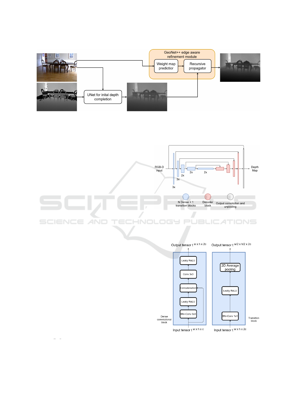
Figure 1: Overview of both modules implemented illustrating the information ﬂow. First, the RGB-D image is used as input

of a U-Net to perform an initial depth completion. The RGB image and the U-Net output are the inputs of the GeoNet++

reﬁnement module (Qi et al., 2020). The RGB component is used to learn a weight map relating the probability of each

pixel to be in the boundaries considering its neighbors. Those weight maps and the intermediary depth images are inputs to a

non-neural module that enhances the ﬁnal prediction.

Our approach relates to (Zhang and Funkhouser,

2018) and (Xian et al., 2020) as we also propose to use

deep neural networks to learn a model and ﬁll in large

missing areas in depth maps provided by low-cost

RGB-D sensors. We also adopted the same dataset

introduced by (Xian et al., 2020) to train our method

and evaluate our results since it contains completed

ground truth depth maps and has statistics reported

for the methods by (Xian et al., 2020) and (Zhang and

Funkhouser, 2018). However, we neither rely on any

external data other than the RGB-D input as done by

(Zhang and Funkhouser, 2018), nor propose an adap-

tive convolution operator to ﬁll in the depth map. In-

stead, we present a simple depth completion architec-

ture that, when guided by a novel loss function de-

signed to stimulate the completion of large missing

areas, could beat the statistics reported by (Zhang and

Funkhouser, 2018).

2 METHOD

2.1 Neural Network Architecture

The depth completion step in Figure 1 is carried out

by the U-Net shown in Figure 2. During the en-

coding phase, the architecture propagates an RGB-D

input tensor through dense convolutional blocks us-

ing LeakyReLU as activation function (with negative

slope equals to 0.01) with batch normalization (BN)

to reduce the internal covariance shift. For an arbi-

trary tensor t

w×h×c

, where w ×h × c represents its di-

mension, each dense convolutional block yields a new

tensor t

×2c

by applying 2c 3x3 ﬁlters and using

average pooling to reduce the spatial dimensions. A

diagram of those components is shown in Figure 3.

Figure 2: Diagram representing the input, the output, and

the blocks used by the U-Net architecture proposed for

depth completion. The number below each blue blocks rep-

resents the multiplicity N of dense blocks allocated before

each transition layer.

Figure 3: Representation of all operations corresponding to

both one dense convolutional block and its following tran-

sition block shown in Figure 2. For all convolutional layers,

we adopted padding equal to one, stride equal to one and 2c

ﬁlters.

VISAPP 2022 - 17th International Conference on Computer Vision Theory and Applications

206

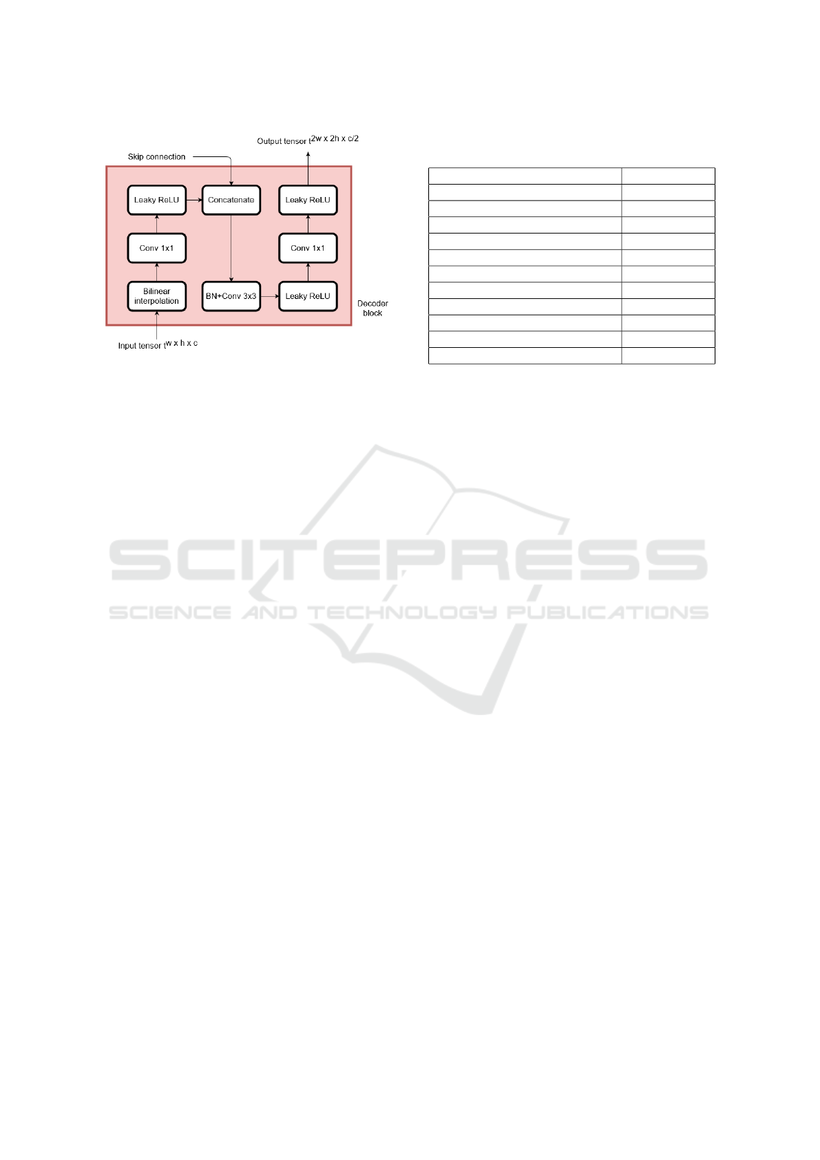
Figure 4: Representation of all operations corresponding to

one decoder block in the U-Net architecture presented in

Figure 2. For all convolutional layers, we adopted padding

equal to one and stride equal to one. Both 1 × 1 convolu-

tional layers have c/2 ﬁlters while the other convolutional

layer has c ﬁlters.

To recover the depth map from the features ex-

tracted in the encoding phase, each decoder block per-

forms a bilinear interpolation on the input tensor and

concatenates the result with another tensor received

by the skipping connection. A diagram of a decoding

block is shown in Figure 4.

Finally, the last block in Figure 2 is composed

of a bilinear interpolation followed by a 3 × 3 con-

volutional layer (eight ﬁlters), a concatenation with

the RGB-D input, another 3 × 3 convolutional layer

(twelve ﬁlters), and then a 1 × 1 convolutional layer

(one ﬁlter) to recover the depth map. Each convolu-

tional layer uses LeakyReLU as the activation func-

tion and considers both padding and stride equal to

one pixel.

The U-Net receives inputs of 544×384×4, corre-

sponding to a centered crop of a 640 ×480 × 4 RGB-

D image from a Microsoft Kinect sensor. We cropped

the input RGB-D data as the depth map has a lower

resolution than the RGB component, which causes

unﬁlled areas at the borders of the depth map. Ta-

ble 1 summarizes the output size for each layer in the

depth completion module.

Once a full depth map is recovered by the U-Net,

we apply the edge-aware reﬁnement module for depth

presented in (Qi et al., 2020). It inputs the RGB com-

ponent to extract its edges using Canny edge detector

and outputs learned weight maps where higher values

correspond to higher probability to be in the bound-

aries considering each one of four possible directions

(top to bottom, bottom to top, left to right, and right

to left).

Then, those weight maps are used to weigh the

depth value for each pixel in the completed depth

Table 1: Output Size for Each Layer in Depth Completion

Network.

Layer Output Size

Input 544 × 384 × 4

Dense + transition block 1 272 × 192 × 8

Dense + transition block 2 136 × 96 × 16

Dense + transition block 3 68 × 48 × 32

Dense + transition block 4 34 × 24 × 64

Dense + transition block 5 17 × 12 × 128

Decoder block 1 34 × 24 × 64

Decoder block 2 68 × 48 × 32

Decoder block 3 136 × 96 × 16

Decoder block 4 272 × 192 × 8

Output convolution + unpooling 544 × 384 × 4

map considering its 4-neighbors. Those maps tend

to have small values in non-boundary regions, which

removes eventual noisy predictions. For boundary ar-

eas, the weight maps present high values that avoid

blurring and preserve sharp predictions. The com-

plete model has approximately 3.8 million parame-

ters, from which only 0.047 million are related to the

reﬁnement module, and the remaining to the depth

completion model.

2.2 EDT Training Loss: Error,

Gradient and SS

We seek to optimize a loss function that combines

three terms to obtain a complete depth representation

using a raw depth map and the RGB image. Our loss

function is similar to the one presented by (Alhashim

and Wonka, 2018), as we adopted the Error, Gradi-

ent and Structural Similarity (SS) terms. Those com-

ponents are not novel and were previously applied in

previous work (Godard et al., 2017; Park et al., 2020;

Ocal and Mustafa, 2020; Shen et al., 2021; Irie et al.,

2019). Our method, however, is the ﬁrst one to use a

distance-transform-based weighing term in each com-

ponent to highlight the contribution of missing areas

during training and improve the ﬁnal results.

2.2.1 Distance Transform Weights

The EDT is applied in binary images to calculate

the distance of all background points to nearest ob-

ject boundaries (Strutz, 2021). We propose to use

the inverted distance transform to weigh the predicted

depth map giving more relevance to pixels located in-

side large missing areas when computing the loss.

Figure 5 shows an example of the EDT calcu-

lated from a raw depth map. By multiplying by ten

and summing one to all values in the obtained dis-

tance transform, we create a weight map (w

edt

) that

Deep Depth Completion of Low-cost Sensor Indoor RGB-D using Euclidean Distance-based Weighted Loss and Edge-aware Reﬁnement

207

Figure 5: Example of a raw depth map (top) and its re-

spective inverted Euclidean distance transform (EDT) from

missing area pixels to the nearest boundary pixel (bottom).

increases the contribution of errors at missing areas,

especially for pixels inside large holes, when comput-

ing the loss functions.

2.2.2 L1 Loss

Considering N predicted depth values (d

pred

) and

their respective completed ground truth depth values

), we calculate the mean absolute error (MAE)

over all samples to compose the ﬁrst term in our

loss function. We adopted the MAE rather than the

root mean squared error during the training phase as

the former is less sensitive to outliers than the latter.

Equation (1) presents the deﬁnition of `

, which cor-

responds to the MAE.

∑

i=1

edt

· (|d

pred

− d

|) (1)

2.2.3 Gradient Loss

To encourage the preservation of accurate object

boundaries in the ﬁnal depth map, we added to our

ﬁnal loss the term `

grad

deﬁned in (2). It averages

the gradient differences in both directions, leading to

small values if the prediction presents edges consis-

tent with the ground truth. To obtain the gradient

components in each direction, we applied the Sobel

Filter.

grad

∑

i=1

edt

(|g

pred

x,i

− g

x,i

| + |g

pred

y,i

− g

y,i

|) (2)

2.2.4 Structural Similarity Loss

The Structural Similarity Index Measure (SSIM)

is another metric for comparing images, especially

when dealing with image degradation (Wang et al.,

2004). To calculate the SSIM, we considered a dy-

namic range of the pixel-values equals to 7500 as

Microsoft Kinect depth maps have pixel values from

500 mm to 8000 mm.

We deﬁne the `

SSIM

as in (3) to adjust its domain

from [−1,1] to [0, 1]. As the SSIM is equal to one

when both images are equal, the equation in (3) also

guarantees that minimizing the loss function leads to

higher SSIM.

SSIM

1 − SSIM(w

edt

pred

edt

)

(3)

2.2.5 Training Loss Function

The equation in (4) describes the loss function

adopted in this work. To balance the contribution of

each term, we set α

= 0.5 and α

= 1000.

training

= `

+ α

· `

grad

+ α

· `

SSIM

(4)

2.3 Training Parameters

We adopted the same parameters described in (Xian

et al., 2020) in order to provide a fair comparison with

our work. We implemented our code using PyTorch

and we trained the model for 100 epochs, using Adam

to optimize our loss function. The batch size was set

as 4 and learning rate was equal to 10

−4

3 RESULTS

The experiments were conducted using an Ubuntu

server equipped with an Intel Core i7-7700K CPU

at 4.20 GHz and two NVIDIA Titan X GPUs, even

though only one GPU was used for both training and

inference. In our experiments, the average inference

time in the test set resulted in approximately 89 FPS.

3.1 Dataset

We adopted the depth completion dataset provided by

(Xian et al., 2020) to conduct our work as it contains

VISAPP 2022 - 17th International Conference on Computer Vision Theory and Applications

208

Table 2: Comparison of the Mean Average Error (MAE) over the test set.

Method Average Error Max Err. Min Err.

(Zhang and Funkhouser, 2018) (CVPR)* 0.170 0.329 0.085

(Xian et al., 2020) (IEEE TASE)* 0.119 0.261 0.037

Ours 0.057 0.255 0.013

Ours (without the reﬁnement module) 0.135 0.342 0.026

∗

as reported by (Xian et al., 2020).

pairs of RGB-D images and their respective complete

ground truth depth maps. The dataset has 3906 im-

ages corresponding to 1302 tuples of RGB, raw depth

map, and ground truth depth map.

We replicated the same training and testing sce-

narios described by (Xian et al., 2020) to conduct our

study. We randomly selected 1083 tuples to compose

the training set and the remaining 219 to be used in the

test set. We performed data augmentation to increase

the number of tuples in training set by horizontally

ﬂipping the selected tuples and permuting the RGB

channels.

3.2 Results of Depth Completion

Figure 6 shows results of depth completion for test

images considering ﬁve repetitions of the recursive

propagator proposed by (Qi et al., 2020) as part of

the edge-aware reﬁnement module.

3.3 Quantitative Evaluation

Even though we considered all pixels of our ground

truth data during the training phase, the errors were

only evaluated on the pixels that had non-zero depth

information measured by the sensor in the input im-

age (Xian et al., 2020; Zhang and Funkhouser, 2018;

Huang et al., 2019; Senushkin et al., 2020). Also, all

depth values were ﬁrst normalized to [0, 1] as done in

(Xian et al., 2020).

Table 2 shows statistics of the MAE for test set

images. We compared the minimum, the maximum

and the average MAE with the values presented by

(Xian et al., 2020). Our method achieved the lowest

errors in these metrics, although smaller errors do not

guarantee better predictions.

Furthermore, we present in Table 2 the results

for the initial depth completion (before the edge-

aware reﬁnement module). Even though the met-

rics for these unreﬁned predictions were not as good

as the ones after the reﬁnement, they were lower

than (Zhang and Funkhouser, 2018) showing the im-

portance of the EDT weights. Also, it was competi-

tive with respect to (Xian et al., 2020), conﬁrming our

U-Net and novel loss function was relevant and im-

proved by reﬁnement module from (Qi et al., 2020).

3.4 Qualitative/Visual Evaluation

We investigated the effect in the ﬁnal model when

weighing (1), (2) and (3) in the training step using the

distance transform. Overall, the model trained with-

out the inﬂuence of the distance transform weights

in loss function terms presented blurred depth maps.

Therefore, the introduction of w

edt

in (1), (2), and

(3) showed inﬂuence to preserve ﬁne details. Figure

7 shows a comparison of outputs generated by two

models of trained using the referred possible scenar-

ios of loss functions.

In addition, we trained four different models vary-

ing by two the number of iterations adopted in the

recursive propagator from three - used by (Qi et al.,

2020) - to nine. We found out that increasing the

number of iterations from three to ﬁve improved our

results, as illustrated in Figure 8. The improvements

for values over ﬁve were not relevant, so we decided

to adopt ﬁve recursive repetitions in our method.

Lastly, Figure 9 presents a comparison of depth

maps obtained before and after applying the edge-

aware reﬁnement module considering the same scenes

shown in Figure 6. Although the U-Net itself could

ﬁll in missing areas, some present a coarse ﬁlling.

Therefore, the edge-aware reﬁnement module has

shown itself a key component to enhance the com-

pleted depth maps and guarantee smooth results in ﬂat

regions and accurate details in borders/edge regions.

4 CONCLUSIONS

This work presents a deep learning method to ﬁll

missing areas in indoor depth maps captured by low-

cost sensors, such as Microsoft Kinect. Our approach

relied only on the original depth map and its respec-

tive RGB image, in contrast to other methods that ex-

ploited external data (Zhang and Funkhouser, 2018;

Huang et al., 2019).

We applied the Euclidean distance transform to

weigh the loss function and increase the inﬂuence of

missing areas when adjusting our CNN’s ﬁlters dur-

ing training. The weighted loss function resulted in

a model that preserves ﬁner details rather than blur-

ring the output depth map when considering the same

Deep Depth Completion of Low-cost Sensor Indoor RGB-D using Euclidean Distance-based Weighted Loss and Edge-aware Reﬁnement

209

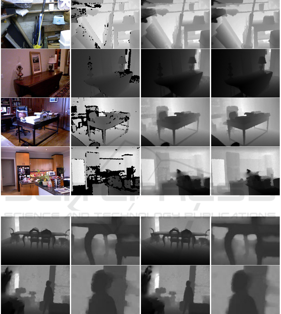
Figure 6: Examples of depth map completed by the proposed method. From left to right: RGB image, raw depth map, output

depth map, and ground truth.

Figure 7: Comparison of the inﬂuence of using the EDT when calculating the loss function over the ﬁnal model. On the

left, we show images generated using the EDT in loss function and a crop of 136 × 96 to highlight ﬁne details. On the right,

we display the results for the same scene removing the term w

edt

in (1), (2), and (3) followed by the same crop previously

mentioned. The loss function using the EDT led to a ﬁnal prediction that tends to preserve details.

inﬂuence for all pixels in the depth map.

Furthermore, by applying a fully-convolutional U-

Net composed of dense blocks followed by the edge-

aware reﬁnement module presented by (Qi et al.,

2020), we could obtain completed depth maps at high

frame rate (89 FPS at inference time) and with met-

rics consistent with other experiments using the same

dataset.

We also investigated the effects of the reﬁnement

module in the ﬁnal results by considering the ini-

VISAPP 2022 - 17th International Conference on Computer Vision Theory and Applications

210

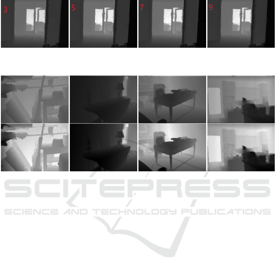
Figure 8: Comparison of complete depth maps for different number of iterations (in red) adopted in the recursive propaga-

tor. The straight line representing the top of the glass door seems better represented from the models using the number of

repetitions greater or equal to ﬁve.

Figure 9: Comparison of depth maps obtained before (top) and after (bottom) the edge-aware reﬁnement module for each

scene in Figure 6. While the outputs of the U-Net present coarse ﬁlling of previously missing areas, the reﬁnement module

boosted the ﬁnal results by keeping sharp edges and smoothing out coarse predictions.

tial depth maps completed only by the U-Net. Even

though the result approximate those reported by (Xian

et al., 2020), the depth maps present coarse results in

some areas. Thus, the edge-aware reﬁnement mod-

ule is an important component to improve numerical

results and present better predictions.

Future studies may consider developing better

methods to generate the initial completed depth map

in order to boost the ﬁnal results. Also, other datasets

containing both raw and ground truth fully com-

pleted depth maps could be proposed and addressed

to provide comparisons between the existing meth-

ods. Lastly, the novel loss function based on inverted

Euclidean distance transform could be applied to train

models in other existing scenarios to exploit its advan-

tages in preserving detail and avoiding unnecessary

blurring of ﬁnal depth maps.

ACKNOWLEDGEMENTS

This study was supported by FAPESP (grant

2019/07316-0). It was also ﬁnanced in part by the Co-

ordination of Improvement of Higher Education Per-

sonnel - Brazil - CAPES (Finance Code 001, grants

88887.136349/2017-00 and 88887.601232/2021-00),

Brazilian National Council for Scientiﬁc and Tech-

nological Development/CNPq (grants 465755/2014-

3, 304266/2020-5) and FAPESP (grant 2014/50851-

0).

REFERENCES

Alhashim, I. and Wonka, P. (2018). High quality monocular

depth estimation via transfer learning. arXiv preprint

arXiv:1812.11941.

Atapour-Abarghouei, A. and Breckon, T. P. (2018). A com-

parative review of plausible hole ﬁlling strategies in

the context of scene depth image completion. Com-

puters & Graphics, 72:39–58.

Bapat, A., Ravi, A., and Raman, S. (2015). An iterative,

non-local approach for restoring depth maps in rgb-d

images. In 2015 Twenty First National Conference on

Communications (NCC), pages 1–6. IEEE.

Chen, L., Lin, H., and Li, S. (2012). Depth image enhance-

ment for kinect using region growing and bilateral ﬁl-

ter. In Proceedings of the 21st International Con-

ference on Pattern Recognition (ICPR2012), pages

3070–3073. IEEE.

de Queiroz Mendes, R., Ribeiro, E. G., dos Santos Rosa,

N., and Grassi Jr, V. (2021). On deep learning tech-

niques to boost monocular depth estimation for au-

Deep Depth Completion of Low-cost Sensor Indoor RGB-D using Euclidean Distance-based Weighted Loss and Edge-aware Reﬁnement

211

tonomous navigation. Robotics and Autonomous Sys-

tems, 136:103701.

Godard, C., Mac Aodha, O., and Brostow, G. J. (2017).

Unsupervised monocular depth estimation with left-

right consistency. In Proceedings of the IEEE con-

ference on computer vision and pattern recognition,

pages 270–279.

Huang, Y.-K., Wu, T.-H., Liu, Y.-C., and Hsu, W. H. (2019).

Indoor depth completion with boundary consistency

and self-attention. In Proceedings of the IEEE/CVF

International Conference on Computer Vision Work-

shops, pages 0–0.

Irie, G., Kawanishi, T., and Kashino, K. (2019). Robust

learning for deep monocular depth estimation. In 2019

IEEE International Conference on Image Processing

(ICIP), pages 964–968. IEEE.

Ocal, M. and Mustafa, A. (2020). Realmonodepth: self-

supervised monocular depth estimation for general

scenes. arXiv preprint arXiv:2004.06267.

Park, J., Joo, K., Hu, Z., Liu, C.-K., and So Kweon, I.

(2020). Non-local spatial propagation network for

depth completion. In Computer Vision–ECCV 2020:

16th European Conference, Glasgow, UK, August 23–

28, 2020, Proceedings, Part XIII 16, pages 120–136.

Springer.

Ponti, M. A., Santos, F. P. d., Ribeiro, L. S. F., and Caval-

lari, G. B. (2021). Training deep networks from zero

to hero: avoiding pitfalls and going beyond. arXiv

preprint arXiv:2109.02752.

Qi, X., Liu, Z., Liao, R., Torr, P. H., Urtasun, R., and Jia,

J. (2020). Geonet++: Iterative geometric neural net-

work with edge-aware reﬁnement for joint depth and

surface normal estimation. IEEE Transactions on Pat-

tern Analysis and Machine Intelligence.

Raviya, K., Dwivedi, V. V., Kothari, A., and Gohil, G.

(2019). Real time depth hole ﬁlling using kinect sen-

sor and depth extract from stereo images. Oriental

journal of computer science and technology, 12:115–

122.

Senushkin, D., Romanov, M., Belikov, I., Konushin, A., and

Patakin, N. (2020). Decoder modulation for indoor

depth completion. arXiv preprint arXiv:2005.08607.

Shen, G., Zhang, Y., Li, J., Wei, M., Wang, Q., Chen,

G., and Heng, P.-A. (2021). Learning regularizer

for monocular depth estimation with adversarial guid-

ance. In Proceedings of the 29th ACM International

Conference on Multimedia, pages 5222–5230.

Silberman, N., Hoiem, D., Kohli, P., and Fergus, R. (2012).

Indoor segmentation and support inference from rgbd

images. In European conference on computer vision,

pages 746–760. Springer.

Strutz, T. (2021). The distance transform and its computa-

tion.

Wang, Z., Bovik, A., Sheikh, H., and Simoncelli, E. (2004).

Image quality assessment: from error visibility to

structural similarity. IEEE Transactions on Image

Processing, 13(4):600–612.

Xian, C., Zhang, D., Dai, C., and Wang, C. C. (2020).

Fast generation of high-ﬁdelity rgb-d images by deep

learning with adaptive convolution. IEEE Transac-

tions on Automation Science and Engineering.

Zhang, Y. and Funkhouser, T. (2018). Deep depth com-

pletion of a single rgb-d image. In Proceedings of

the IEEE Conference on Computer Vision and Pattern

Recognition, pages 175–185.

VISAPP 2022 - 17th International Conference on Computer Vision Theory and Applications

212