Image Quality Assessment using Deep Features for Object Detection

Poonam Beniwal, Pranav Mantini and Shishir K. Shah

Quantitative Imaging Laboratory, Department of Computer Science, University of Houston,

4800 Calhoun Road, Houston, TX 77021, U.S.A.

Keywords:

Object Detection, Image Quality, Video Compression, Video Surveillance.

Abstract:

Applications such as video surveillance and self-driving cars produce large amounts of video data. Computer

vision algorithms such as object detection have found a natural place in these scenarios. The reliability of

these algorithms is usually benchmarked using curated datasets. However, one of the core challenges of

working with computer vision data is variability. Compression is one such parameter that introduces artifacts

(variability) in the data and can negatively affect performance. In this paper, we study the effect of compression

on CNN-based object detectors and propose a new full-reference image quality metric based on Discrete

Cosine Transform (DCT) to quantify the quality of an image for CNN-based object detectors. We compare

this metric with commonly used image quality metrics, and the results show that the proposed metric correlates

better with object detection performance. Furthermore, we train a regression model to estimate the quality of

images for object detection.

1 INTRODUCTION

Video surveillance cameras are being deployed in

large numbers to ensure safety and security. Large

infrastructures, such as airports and shopping malls,

employ thousands of cameras and generate massive

amounts of data. Since it is impossible to review such

amounts of data manually, automatic video analytic

systems are utilized to accomplish tasks such as ob-

ject detection, tracking, anomaly detection, etc. Video

analysis is generally performed at a centralized loca-

tion. Video from the camera is transmitted to a cen-

tral location over data channels. Since these channels

have limited bandwidth, video compression is used to

realize this framework. However, this introduces ar-

tifacts in the data that can affect the performance of

vision algorithms and make automated systems less

reliable. Many other factors, e.g., weather, illumina-

tion, etc., affect performance. This paper focuses on

compression artifacts common in video surveillance

systems and their effect on CNN-based object detec-

tion algorithms.

H.264 (Wiegand et al., 2003) is the most com-

monly used compression algorithm in surveillance

cameras. It uses motion prediction, motion com-

pensation, quantization, etc., to achieve high com-

pression ratios. It is more complicated than image

compression algorithms like JPEG (Wallace, 1992),

where only spatial information is utilized for com-

pression. The primary objective of the compression

algorithm is to reduce the amount of data that needs to

be transmitted or stored, which generally comes with

the loss of data quality. It directly impacts perfor-

mance and often decreases the performance and relia-

bility of computer vision algorithms. Figure 1 shows

object detection results on an image compressed us-

ing different compression parameter.

Image quality assessment (IQA) algorithms have

been studied for a long time. However, these algo-

rithms were designed with the intent of measure im-

pact on human perceptual ability. In doing so, the

quality of an image is determined by the mean of

opinion score (MOS) assigned by humans (Zhai and

Min, 2020). With increased vision applications, al-

gorithms are the end recipients of images and videos.

As a result, there has been a signiﬁcant effort in the vi-

sion community to determine image quality for algo-

rithms. For example, face image quality assessment

(FIQA) (Schlett et al., 2020) focuses on assessing the

quality of images for face recognition. The quality of

a face image determines how good the image is for

recognition. In other words, the image quality cor-

relates with the face recognition algorithm’s perfor-

mance. A high-quality image implies that the algo-

rithm would perform well on the image, and a low-

quality implies that the algorithm may fail to recog-

nize face in the image.

In this paper, we focus on understanding the image

quality for object detection algorithms. The quality

of an image should determine its suitability for object

detection and its expected performance. Object de-

706

Beniwal, P., Mantini, P. and Shah, S.

Image Quality Assessment using Deep Features for Object Detection.

DOI: 10.5220/0010917000003124

In Proceedings of the 17th International Joint Conference on Computer Vision, Imaging and Computer Graphics Theory and Applications (VISIGRAPP 2022) - Volume 4: VISAPP, pages

706-714

ISBN: 978-989-758-555-5; ISSN: 2184-4321

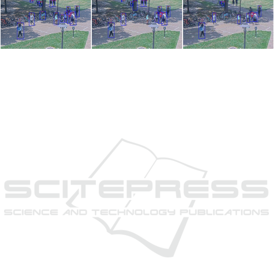
Figure 1: Figure shows object detection results on a sample frame from a video. (Left) Frame is from a video that is

uncompressed. All the objects in the images are detected. (Middle) There are 4 objects that are not detected after applying

low compression. (Right) The number of objects that are not detected has increased with increased compression.

tection is a core vision algorithm, and its results are

used in a broad range of other applications like ob-

ject tracking, anomaly detection, etc. Assessing the

image quality for object detection can be a difﬁcult

task as it involves ﬁnding the location of objects in the

image and classifying them. Many factors affect the

performance of object detectors, but in this work, we

focus primarily on the effect of compression in video

surveillance scenarios.

Recent methods in FIQA use performance-based

labels to assign quality labels to images. But directly

using these ideas is not suitable for determining the

quality of an image for object detection. We make

two important contributions in this paper. First, we

propose a new quality metric based on the output from

intermediate layers of CNN models for object detec-

tion. The proposed metric is validated by checking

its correlation with object detection performance and

comparing it with other widely used image quality

metrics. Second, we train a regression model to esti-

mate the quality of compressed images for object de-

tection. We evaluate our approach on a comprehen-

sive surveillance video dataset with indoor and out-

door scenarios to infer the efﬁcacy of the metric and

the prediction model.

The rest of the paper is organized as follows: The

second section describes the related work. The third

section discusses the limitation of performance-based

metrics and the idea behind the proposed metric and

regression model. The section is followed by discus-

sion of dataset and experimental settings. A predic-

tion model is deﬁned in the next section.

2 RELATED WORK

Image quality assessment methods have received sig-

niﬁcant interest from the vision community (Zhai and

Min, 2020). Initially, the focus was on image quality

from the perspective of the human visual system. But

in recent years, image quality has been determined

for various purposes such as face recognition, the aes-

thetic quality of images, etc.

Image Quality Assessment. A detailed survey of

IQA methods is conducted in (Zhai and Min, 2020).

Recent methods utilize deep learning models to ac-

complish image quality assessment. These methods

(Yang et al., 2019) can be divided into patch-based

and image-based categories. Patch-based methods di-

vide an image into patches and estimate quality as an

agglomeration value of quality of individual patches.

An end-to-end optimized method is proposed in (Ma

et al., 2017) where the network is divided into two

sub-networks. The ﬁrst one is trained on a large-scale

dataset to identify the type of distortion. The latter

uses the output of the ﬁrst network to predict quality.

Gao et al. (Gao et al., 2018) extract features from dif-

ferent layers of models to identify and then obtain a

better quality score.

Image Quality for Vision Algorithms: Schlett et al.

(Schlett et al., 2020) surveyed the progress in FIQA.

Chen et al. (Chen et al., 2014) extracted different

features from the input image and computed the ﬁ-

nal quality score as the weighted sum of the score ob-

tained from each feature. Rowden (Best-Rowden and

Jain, 2017), (Best-Rowden and Jain, 2018) presented

5 different variants of face image quality assessment.

In their experiment, three quality scores for ground

truth data are determined by human assessment. In

one variant, a face recognition model was used to de-

termine the quality of the image. Face embedding is

used in the face recognition model and quality assess-

ment models. Shi et al. (Shi and Jain, 2019) proposed

to compute probabilistic metrics where mean of em-

bedding is used as feature representation, and vari-

ance is used as a quality indicator. SER-FIQ uses a

similar approach (Terhorst et al., 2020) where the sig-

moid of negative Euclidean distance between every

pair of embedding is used to determine the quality of

the image. Embeddings for an image are obtained by

using dropout.

There is limited work available for assessing the

quality of images for object detection. A no-reference

model (Kong et al., 2019) has been proposed to pre-

dict the quality of images for object detection. An

image compression algorithm was used to compress

individual frames of a video. They proposed a metric

Image Quality Assessment using Deep Features for Object Detection

707

that was a variant of frame detection accuracy com-

monly used to measure pedestrian detection perfor-

mance. A regression model based on a bagging en-

semble of regression trees was used to train the model.

Instead of using a performance-based model, we pro-

posed a new metric that utilizes DCT of features ob-

tained from a convolutional neural network (CNN).

We mainly focus on the quality of compressed videos

from video surveillance cameras. Videos are com-

pressed using a video compression algorithm. DCT

on the output of convolutional layer has been used be-

fore by Ghosh et al.. In their work, the idea behind

using DCT was for early convergence and obtaining

sparse matrix weight for CNN. In our work, we are

using DCT on features to ﬁnd the information loss.

3 METHOD

In recent face quality assessment algorithms (Schlett

et al., 2020), performance-based metrics are used

to assign quality labels to images. But using per-

formance metrics as labels is not as simple in ob-

ject detection. We are describing below why using

performance-based labels or compression parameters

can result in poor quality labels.

• Object detection is a classiﬁcation as well as a

localization problem. It locates one or more ob-

jects present in the image and identiﬁes the class

of each object. The output is a bounding box

and classiﬁcation score for each detected object.

Performance is deﬁned based on conﬁdence score

and Intersection over Union (IoU) with ground-

truth. Using an average classiﬁcation score, av-

erage IoU, or a combination of both does not re-

sult in suitable labels. There are two problems

with this. First, deep learning-based object detec-

tors are miscalibrated (Guo et al., 2017) and show

overconﬁdence in prediction. Second, the aver-

age classiﬁcation or localization score (IoU) does

not consider missed detections, a common prob-

lem with increased compression.

• Average precision (AP) is the commonly used per-

formance metric in object detection. It takes into

consideration the precision and recall of detection

results. But it is not a good measure for a single

image or frame of a video. Figure 2 shows ob-

ject detection results on a frame of a video that

is subject to two different levels of compression,

low and high. Low compressed image has double

detection resulting in False Positives (FP), but the

high compressed image has False negatives (FN).

AP for both images is approximately the same de-

Figure 2: Figure shows result of Faster RCNN (Ren et al.,

2015) object detection model on a low compressed frame

(top) and highly compressed frame (bottom).

spite having very different detection results. Us-

ing AP as the quality label will assign the same

score to both images. Assigning the same quality

label to both images will not be right as the loss

in information caused FN while FP is mainly be-

cause of the detector’s miscalibration.

• Object detectors show low performance on im-

ages (Ren et al., 2015) containing small objects

and occluded objects. The lower performance

in such scenarios is because of object detectors’

properties and not always the result of compres-

sion. Since our primary focus is on information

loss because of compression, the quality metric

should not consider object detector biases.

Because of these limitations, instead of using the

performance-based metrics, we proposed a new met-

ric for assigning labels to the frames of a video. In

this paper, we use the term image to refer to a video

frame.

3.1 Modeling Quantization Error from

H.264 Compression

H.264 uses intra-frame and inter-frame prediction to

reduce the information redundancy in spatial and tem-

poral domains. A block diagram of the compression

procedure is shown in Figure 3. A frame of video

is divided into macro-blocks. Motion estimation and

prediction are used to predict a macro-block. The

difference between predicted and actual macro-block

is used to calculate the residual block. This step is

known as motion compensation. Let B

be the origi-

nal block, and let B

be the predicted block, then the

VISAPP 2022 - 17th International Conference on Computer Vision Theory and Applications

708

residual block B

is deﬁned as

= B

−B

(1)

The residual is transformed using an approxima-

tion of DCT, called Integer Transform, to obtain the

frequency coefﬁcients. These coefﬁcients are quan-

tized and rounded to the nearest integer. This op-

eration results in loss of information that cannot be

inverted. The amount of quantization is deﬁned by

Quantization Parameter (QP). Let q be the quantiza-

tion parameter. Then the quantized coefﬁcients Q are

obtained as:

Q = Round(

DCT (B

)

) (2)

A bitstream encoding (E) is applied to the Q and

then encoded data is transmitted. The decoder does

the inverse of the encoder process to obtain the quan-

tized coefﬁcients. Note that the encoding is a lossless

invertible process.

Q = E

−1

(E(Q)) (3)

Initially, the received quantized coefﬁcients are in-

verse scaled with q and then the inverse transform is

applied to reconstruct the residual block. Let

the reconstructed residual block,

= DCT

−1

(Q ∗q) (4)

The reconstructed residual block and predicted

block are added to get the compressed block. The pre-

dicted block is identical to the one used at the encoder.

The reconstructed block (compressed) B

is obtained

+ B

(5)

The reconstructed block has undergone loss in

quality due to quantization and rounding in the en-

coding process, which are non-invertible operations.

We hypothesize that a measure of image quality can

be attributed to the amount of quantization error that

has occured during the H.264 encoding-decoding pro-

cess. From equation 2 and 4, we have:

DCT (

) = Round(

DCT (B

)

) ∗q. (6)

Considering that DCT is a linear operation, from

equation 5, we have:

DCT (B

) = Round(

DCT (B

)

) ∗q + DCT (B

). (7)

In general a compression loss occurs for q > 1. If

we consider rounding to be a rounding down opera-

tion of round(a/q) ∗q, we have a ≥ round(a/q) ∗q

for q > 1. Using round operation properties, we have:

Figure 3: Figure shows block diagram of video encoding

and decoding step for H.264 compression.

DCT (B

) ≤ (Round(

DCT (B

)

) + Round(

DCT (B

)

)) ∗q.

(8)

Since round(a + b) ≤ round(a) + round(b), we

have:

DCT (B

) ≤ (Round(

DCT (B

) + DCT (B

)

)) ∗q.

(9)

So the relation between the DCTs of the com-

pressed block and original is given by:

DCT (B

) ≤ Round(

DCT (B

)

) ∗q. (10)

An estimate of the quantization error can be ob-

tained by computing

DCT (B

)

DCT (B

)

. (11)

From Equation 11, we observe that a measure of

the quantization error involved in the H.264 process

can be obtained by consider the ratio of the DCT’s of

the original and reconstructed image blocks.

3.2 Quantifying Loss in Information in

CNNs due to H.264 Compression

Deep learning algorithms have shown signiﬁcant im-

provements in the performance of object detection

tasks. Convolutional Neural Networks (CNNs) are at

the heart of these methods and are used for feature

extraction, localization, and classiﬁcation. A convo-

lution operation is applied using a ﬁlter followed by

an activation function. CNNs learn a set of ﬁlters via

optimization process. These ﬁlters extract important

information from images by applying the following

operation

I(x,y)~ h =

L/2

∑

i=−L/2

L/2

∑

j=−L/2

I(x+L/2, y+L/2)∗h(i, j),

(12)

where ~ is convolution operation, I is the image and

f is a CNN ﬁlter of size 2L+1. Note that while these

Image Quality Assessment using Deep Features for Object Detection

709

Figure 4: Figure (Left) shows the block diagram for proposed quality metric. Features from original and compressed images

are extracted using backbone of an object detector model. The ration of DCT of extracted original and compressed features

is used as quality label. (Right) Figure shows the regression model used to predict quality labels. A random patch from the

compressed image is given as input to the prediction label.

are referred to as convolution functions, the operation

actual computes the correlation between the image

function I and ﬁlter h.

Our metric is based on the assumption that com-

pression artifacts will change features extracted from

images. There are activations at background areas

with increased compression and no activations for

some objects present in the image.

Let us consider a 1D function f ∈R

1XN

and a ﬁlter

h. If we consider the type-II periodic extension of the

function f

∈ R

1X2N

, we have

(n) = f [((n))

] + f [((−n −1))

]

∀ k ∈ [0,1,...,2N −1].

(13)

We know that DCT can be expressed in terms of

the 2N point Fourier transform as:

(k) = cF

(k) ∀ k ∈ [0, 1,..N −1], (14)

where c = exp(−jπk/2N), j is the complex number

(

√

−1), F

(k) is DCT of f and F

(k) is the Fourier

transform of f

If we consider the Fourier transform of the corre-

lation between f

and a ﬁlter h, by correlation theo-

rem we have,

F ( f

~ h)(k) = F

(k).H

∗

(k)

∀ k ∈ [0,1,..N −1],

(15)

where F (.) is the Fourier transform, (∗) is the conju-

gate and H(k) is the Fourier transform of h.

Now if we consider the periodic extension of an

H.264 reconstructed image block B

(with twice the

number of rows and columns) and its correlation with

a ﬁlter h, i.e., the output of convolution layer in the

CNN based object detector,

F (B

~ h)(u,v) = F (B

)(u,v).H

∗

(u,v)

∀ (u,v) ∈ [0,1,..N −1].

(16)

From equation 14, we can express the Fourier

transform in terms of the DCT, as

F (B

~ h) = 1/c

∗DCT (B

).H

∗

∀ (u,v) ∈ [0,1,..N −1],

(17)

where c

is a constant. For ease of reading, we avoid

using (u,v) in the following equations. All function

that follow can be assumed to be functions of fre-

quency (u,v).

From equation 10,

F (B

~ h) = 1/c

Round(

DCT (B

)

).qH

∗

∀ (u,v) ∈ [0,1,..N −1].

(18)

This can be rewritten as:

F (B

~ h) ≤ 1/c

Round(

DCT (B

).H

∗

q.H

∗

)

∗q.H

∗

(19)

=⇒ ≤ 1/c

Round(

F(B

~ h)

q.H

∗

) ∗q.H

∗

(20)

Considering the similarity between equation 10

and 20, we infer that the loss in information due to

the quantization of a DCT block with a quantization

value of q has the effect of quantizing the 2N point

DFT of the output from the ﬁrst layer of CNN (with a

ﬁlter H) with a quantization value of (q.H∗).

Similar to equation 11, the loss in information due

to the quantization error in the H.264 process can be

estimated as:

F(B

~ h)

F(B

~ h)

. (21)

3.3 Metric Computation

In H.264 compression process, images are trans-

formed to YCbCr color space before encoding. Since

YCbCr is a linear combination of RGB channels; we

ignore this and compute the metric on RGB images.

Each block in the image undergoes a different amount

of quantization depending on the content. However,

quality is usually expressed as an accumulated mean

of these quantization values. To account for this, we

compute the metric on complete images instead of

processing each block.

VISAPP 2022 - 17th International Conference on Computer Vision Theory and Applications

710

Furthermore, convolution layer has multiple ﬁl-

ters. In our work, the ratio is calculated for each ﬁlter

of the ﬁrst convolutional layer of the deep neural net-

work. To get a single score representing the image’s

quality, we use the mean of the above-deﬁned ratio for

all ﬁlters as a quality label. Figure 4 shows the block

diagram of obtaining training labels of an image.

In this work, we are using Faster-RCNN (Ren

et al., 2015) backbone for feature extraction. Faster-

RCNN network backbone is a ResNet network that

is pre-trained on image classiﬁcation dataset and then

ﬁne-tuned on COCO (Lin et al., 2014) dataset. The

network helps to select features that are relevant to

object detection.

4 EXPERIMENTS

4.1 Dataset

In this paper, we are using videos collected from

video surveillance scenarios (Aqqa et al., 2019). We

used 11 videos consisting of 5 different scenes, in-

cluding indoor and outdoor scenarios. The dataset

is compressed using H.264 using 4 bandwidths and

5 constant rate factor (CRF) values to obtain videos

showing variations in quality. For each video, there

are 20 compressed variants. There are 10 videos of

average length 5 minutes and 1 video of length 2 min-

utes 30 seconds. The dataset has a total of 92890

frames. The resolution of 7 videos is 1920*1080, and

4 videos are of resolution 1080 ∗584.

4.2 Evaluation

The idea behind the proposed metric is to assign

quality labels to images. Higher values indicate

higher quantization loss and lower quality. Con-

versely, lower values imply better quality. We com-

pute the correlation between the proposed metric and

object detection performance metric, AP, to validate

the proposed quality metric. AP is not well deﬁned

for individual frames so we calculate it over the non-

overlapping window of 100 frames in each video. In

this paper, we are using Faster-RCNN (Ren et al.,

2015) for object detection.

Since our metric is deﬁned for each frame, a mean

of quality over 100 frames is used to assign quality

label for that window. Table 1 shows a comparison

of 6 commonly used quality metrics (Beniwal et al.,

2019) and their correlation with object detection per-

formance metric. Of the six metrics, two are full-

reference metrics, and four are no-reference quality

metrics. SSIM (Wang et al., 2004), and PSNR are

Table 1: Table shows the correlation between quality met-

rics and AP.

Metric LCC SRCC KRCC

Contrast 0.050 0.180 0.168

Noise 0.102 0.074 0.047

Blur 0.221 0.143 0.089

PSNR 0.627 0.695 0.508

Blockiness 0.627 0.670 0.491

SSIM 0.650 0.614 0.440

Proposed metric 0.701 0.693 0.503

Table 2: Table shows the correlation between quality met-

rics and AP. (Top) table shows results on subset of dataset

that includes videos compressed using CRF-35, CRF-41,

CRF-47. (Bottom) table shows results on subset of data that

includes video compressed at CRF-41, CRF-47.

Metric LCC SRCC KRCC

Contrast 0.015 0.147 0.138

Noise 0.089 0.066 0.044

Blur 0.160 0.141 0.089

PSNR 0.564 0.604 0.431

Blockiness 0.514 0.570 0.403

SSIM 0.549 0.527 0.431

Proposed metric 0.626 0.640 0.447

Metric LCC SRCC KRCC

Contrast 0.026 0.111 0.106

Noise 0.102 0.041 0.021

Blur 0.044 0.045 0.027

PSNR 0.427 0.461 0.320

Blockiness 0.307 0.390 0.262

SSIM 0.378 0.375 0.25

Proposed metric 0.498 0.511 0.337

full-reference metrics that are commonly used for de-

termining image quality. Blockiness is a no-reference

metric that uses the ratio of differences in luminance

of pixels in inter and intra-pairs. Blur (Mu et al.,

2012) focuses on spatial artifacts introduced because

of the removal of high-frequency components. The

detail of metric noise is given in (Janowski and Pa-

pir, 2009). Contrast shows how distinguishable the

objects are from the background.

We used Pearson linear correlation coefﬁcient

(LCC), Spearman’s rank correlation coefﬁcient

(SRCC), and Kendall’s rank correlation coefﬁcient

(KRCC) to validate the proposed metric. In Table 1,

our proposed metric shows higher LCC values com-

pared to other metrics. SRCC and KRCC values for

PSNR and the proposed metric are very close. The

results are calculated over the complete dataset.

Aqqa et al. (Aqqa et al., 2019) showed that ob-

ject detection model’s performance dropped at higher

Image Quality Assessment using Deep Features for Object Detection

711

Table 3: Table shows the performance of prediction method on videos from the dataset.

Scene Video LCC SROCC KRCC MSE MAE

Inside Scene 1

Inside Library 1 0.594 0.778 0.591 6.549 3.515

Inside Library 2 0.560 0.772 0.584 6.588 3.621

Inside Library 4 0.600 0.794 0.606 6.514 4.170

Outside

Scene 2

Outside Library 4 0.546 0.806 0.629 6.187 3.005

Outside Library 5 0.530 0.801 0.624 6.307 2.986

Outside Library 6 0.559 0.794 0.615 6.684 3.156

Scene 3

Library 6 0.405 0.707 0.523 5.484 2.327

Library 11 0.411 0.692 0.506 5.331 2.359

Dataset 0.574 0.789 0.610 6.197 3.049

Table 4: Table shows the performance of regression model on scenes that were not seen during training.

Scene Video LCC SROCC KRCC MSE MAE

Inside Scene 1

Student Center 1 0.408 0.644 0.461 5.972 4.081

Student Center 4 0.410 0.654 0.470 6.323 4.576

Outside Scene 2 campus 1 0.517 0.730 0.535 7.038 3.634

Dataset 0.490 0.673 0.486 6.453 4.101

compression. We created two subsets of the dataset to

analyze correlation further. The ﬁrst subset includes

video compressed at CRF-35, CRF-41, and CRF-47.

The second subset has video compressed with CRF-

41 and CRF-47. The correlation results are shown

in Table 2. The results show the drop in correlation

for all metrics with increased compression. But, our

metric shows relatively lower drop than the other met-

rics. With an increase in compression, object detec-

tion models show high detection variation between

consecutive frames. One reason can be the loss of

important information because of compression that

makes an object more detectable. It is difﬁcult to

capture the variation in quality between consecutive

frames of a video by quality metrics. But, the pro-

posed quality metric shows relatively less decrease in

correlation at higher compression. These results vali-

date the idea that the proposed metric provides a cor-

relation between image quality and object detection

performance.

While metrics such as PSNR and Blockiness also

show a high correlation to the AP, these are com-

puted independent of properties of the object detec-

tion model. A model trained to extract better features

from the image will change performance. Our metric

is dependent on the features extracted from the deep

learning models and will vary based on features. But,

the value of PSNR and Blockiness would remain the

same. Since our goal is to determine the performance

of algorithms, quality should change with the algo-

rithm. This makes the proposed metric more appro-

priate.

5 PREDICTION

The proposed metric is a full-reference metric de-

ﬁned based on features from original and compressed

videos. In real-world scenarios, uncompressed im-

ages are not available for each image. The perfor-

mance of vision algorithms needs to be determined

based on the compressed image. In this section, we

develop a model that predicts the quality of images.

The predicted quality correlates with object detection

models’ performance.

5.1 Model

We trained a regression model to predict the quality

of an image. A network inspired by AlexNet architec-

ture (Krizhevsky et al., 2012) is used for our regres-

sion model. It includes 5 convolutional layers and 4

fully-connected layers. The network is not pre-trained

on any other dataset.

Input to the network is a 224*224 patch from the

image. Although we are using the original images

to obtain the quality label, the regression model only

needs compressed images for predicting image qual-

ity. The model is trained with SGD optimizer and

mean squared error loss function. The network is

trained for 50 iterations.

Videos are obtained from ﬁxed cameras with a

constant background. It can create a bias towards

the background features. We perform regularization

through data augmentation to avoid this, allowing the

VISAPP 2022 - 17th International Conference on Computer Vision Theory and Applications

712

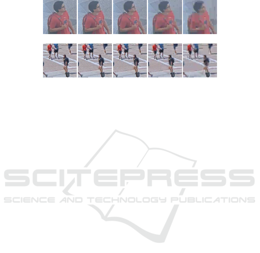
Quality=12.81 Quality=12.68 Quality=14.80 Quality=17.14 Quality=18.08

Quality=9.43 Quality=9.22 Quality=10.22 Quality=12.77 Quality=15.83

Figure 5: Figure shows image quality for frame of video compressed using different compression parameter. Each row

shows patch from frame of a video. Each column shows the images compressed with same compression parameter. CRF-23,

CRF-29, CRF-35, CRF-41, CRF-47 are compression parameters for each column respectively.

model to learn features related to compression arti-

facts. We randomly select a 224 ∗224 patch from the

image to extract training features, and the label for

the patch is the quality computed for the image. Dur-

ing testing, we need to sample patches to calculate

the metric. Depending on the image features, patches

from the same image can produce different quality

metrics. It is imperative to select patches that con-

tribute the most towards the feature extraction process

in the CNN layers. These tend to be locations in the

feature maps that are extracted from the intermediate

layers and produce either a high or low value in ac-

tivation. We take activation maps from intermediate

layers, construct a 2D probability map using a non-

parametric approach, and sample points to localize

patches that contribute the most towards the feature

extraction process. We select two patches from the

image, pass them through the regression model, and

compute the quality of the image as a mean of the re-

gression values obtained. We selected 8 videos from

3 different scenes to train our model. We randomly

selected 26240 frames from the dataset. The dataset

contains compressed images with 4 bandwidths and 5

CRFs values. The rest of the data is used for testing.

5.2 Evaluation

Following evaluation metrics that are commonly used

to quantify the performance of regression models, we

use Mean Squared Error (MSE), Mean Absolute Er-

ror (MAE), LCC, SROCC and KCC to understand the

performance of the prediction model. A higher value

of correlation implies good performance. The results

are summarized in Table 3. As shown in Table, the

predicted values correlate with ground-truth labels of

quality. The videos from library scene show less cor-

relation as compared to other metrics. These videos

contain 1 or 2 objects in a frame. The objects are of

smaller size as compared to other videos. The amount

of compression is less as compared to other videos.

Figure 5 shows the prediction result for images com-

pressed at different compression levels. With increase

in compression, the quality value increases. Increase

in proposed metric value indicates higher quantization

loss and poor image quality.

In our methods, we need uncompressed and com-

pressed images to assign quality labels to images. Ob-

ject detection datasets e.g. COCO dataset (Lin et al.,

2014) and Pascal object dataset (Everingham et al.,

2010) have images collected from different sources

and are already compressed. Instead of using a differ-

ent dataset, we excluded 2 scene containing 3 videos

from the training data. The excluded video contains

both indoor and outdoor scenarios. We evaluated our

regression model on these 3 videos and results are

shown in Table 4. The results show that videos from

indoor scenarios show a lower correlation than other

videos. Video showing poor performance has objects

of small size, and lighting conditions are really dif-

ferent compared to videos used for training. It can

make generalization difﬁcult and result in poor per-

formance. MSE and MAE values show the difference

between predicted and correct values. Higher values

imply less accurate predictions. The difference be-

tween MAE and MSE loss suggest that we can use

the model on unseen videos.

6 CONCLUSION

In this paper, we proposed a quality metric based on

the features extracted from deep learning models. The

proposed metric correlates with object detection mod-

els’ performance. The results show that the proposed

Image Quality Assessment using Deep Features for Object Detection

713

metric correlates better at higher compression than

SSIM and PSNR. One advantage of our metric is that

it depends on both image and model used for feature

extraction. The metric will change based on features

extracted from images. In the future, we will focus on

determining the quality of image patches.

ACKNOWLEDGEMENTS

This work was supported in part by Grant No.

60NANB17D178 from U.S. Dept. of Commerce, Na-

tional Institute of Standards and Technology.

REFERENCES

Aqqa, M., Mantini, P., and Shah, S. K. (2019). Understand-

ing how video quality affects object detection algo-

rithms. In VISIGRAPP (5: VISAPP), pages 96–104.

Beniwal, P., Mantini, P., and Shah, S. K. (2019). Assessing

the impact of video compression on background sub-

traction. In Asian Conference on Pattern Recognition,

pages 105–118. Springer.

Best-Rowden, L. and Jain, A. K. (2017). Automatic

face image quality prediction. arXiv preprint

arXiv:1706.09887.

Best-Rowden, L. and Jain, A. K. (2018). Learning

face image quality from human assessments. IEEE

Transactions on Information forensics and security,

13(12):3064–3077.

Chen, J., Deng, Y., Bai, G., and Su, G. (2014). Face image

quality assessment based on learning to rank. IEEE

signal processing letters, 22(1):90–94.

Everingham, M., Van Gool, L., Williams, C. K., Winn, J.,

and Zisserman, A. (2010). The pascal visual object

classes (voc) challenge. International journal of com-

puter vision, 88(2):303–338.

Gao, F., Yu, J., Zhu, S., Huang, Q., and Tian, Q. (2018).

Blind image quality prediction by exploiting multi-

level deep representations. Pattern Recognition,

81:432–442.

Guo, C., Pleiss, G., Sun, Y., and Weinberger, K. Q. (2017).

On calibration of modern neural networks. In Interna-

tional Conference on Machine Learning, pages 1321–

1330. PMLR.

Janowski, L. and Papir, Z. (2009). Modeling subjective

tests of quality of experience with a generalized linear

model. In 2009 International Workshop on Quality of

Multimedia Experience, pages 35–40. IEEE.

Kong, L., Ikusan, A., Dai, R., and Zhu, J. (2019). Blind im-

age quality prediction for object detection. In 2019

IEEE Conference on Multimedia Information Pro-

cessing and Retrieval (MIPR), pages 216–221. IEEE.

Krizhevsky, A., Sutskever, I., and Hinton, G. E. (2012). Im-

agenet classiﬁcation with deep convolutional neural

networks. Advances in neural information processing

systems, 25:1097–1105.

Lin, T.-Y., Maire, M., Belongie, S., Hays, J., Perona, P.,

Ramanan, D., Doll

ar, P., and Zitnick, C. L. (2014).

Microsoft coco: Common objects in context. In Euro-

pean conference on computer vision, pages 740–755.

Springer.

Ma, K., Liu, W., Zhang, K., Duanmu, Z., Wang, Z., and

Zuo, W. (2017). End-to-end blind image quality as-

sessment using deep neural networks. IEEE Transac-

tions on Image Processing, 27(3):1202–1213.

Mu, M., Romaniak, P., Mauthe, A., Leszczuk, M.,

Janowski, L., and Cerqueira, E. (2012). Framework

for the integrated video quality assessment. Multime-

dia Tools and Applications, 61(3):787–817.

Ren, S., He, K., Girshick, R., and Sun, J. (2015). Faster

r-cnn: Towards real-time object detection with region

proposal networks. Advances in neural information

processing systems, 28:91–99.

Schlett, T., Rathgeb, C., Henniger, O., Galbally, J., Fier-

rez, J., and Busch, C. (2020). Face image qual-

ity assessment: A literature survey. arXiv preprint

arXiv:2009.01103.

Shi, Y. and Jain, A. K. (2019). Probabilistic face embed-

dings. In Proceedings of the IEEE/CVF International

Conference on Computer Vision, pages 6902–6911.

Terhorst, P., Kolf, J. N., Damer, N., Kirchbuchner, F., and

Kuijper, A. (2020). Ser-ﬁq: Unsupervised estimation

of face image quality based on stochastic embedding

robustness. In Proceedings of the IEEE/CVF Con-

ference on Computer Vision and Pattern Recognition,

pages 5651–5660.

Wallace, G. K. (1992). The jpeg still picture compression

standard. IEEE transactions on consumer electronics,

38(1):xviii–xxxiv.

Wang, Z., Lu, L., and Bovik, A. C. (2004). Video quality as-

sessment based on structural distortion measurement.

Signal processing: Image communication, 19(2):121–

132.

Wiegand, T., Sullivan, G. J., Bjontegaard, G., and Luthra,

A. (2003). Overview of the h. 264/avc video coding

standard. IEEE Transactions on circuits and systems

for video technology, 13(7):560–576.

Yang, X., Li, F., and Liu, H. (2019). A survey of dnn meth-

ods for blind image quality assessment. IEEE Access,

7:123788–123806.

Zhai, G. and Min, X. (2020). Perceptual image quality as-

sessment: a survey. Science China Information Sci-

ences, 63(11):211301.

VISAPP 2022 - 17th International Conference on Computer Vision Theory and Applications

714