Exploring Classification in Open and Closed Eyes EEG Data for

People with Cognitive Disorders

Ioanna Chouvarda

, Lampros Mpaltadoros

, Ioanna Boutziona

, George Nikolaos Tsakonas

Magda Tsolaki

and Konstantinos Diamantaras

Lab of Computing Medical Informatics and Biomedical Imaging Technologies, School of Medicine,

Aristotle University of Thessaloniki, Greece

Greek Alzheimer Association, Thessaloniki, Macedonia, Greece

Department of Information and Electronic Engineering, International Hellenic University, Thessaloniki, Greece

Keywords: Alzheimer’s Disease, Mild Cognitive Impairment, EEG, Signal Processing, Machine Learning.

Abstract: Cognitive disorders, including Alzheimer’s Disease (AD), are health issues concerning all society. The

evolution of technology and Artificial Intelligence (AI)/ Machine Learning (ML) in the health domain

promises an earlier and more accurate diagnosis for Alzheimer’s disease and Dementia. In this study, we

examine Healthy patients and patients with AD and Mild Cognitive Impairment (MCI), often a prior step of

AD. With the use of EEG, we collect data from their brain activity. After a basic processing step, kernel PCA

is applied as a dimensionality reduction method using segments of the multichannel signal, and the

transformation output is employed as input for the predictive model. Machine learning functions are used to

classify data correctly into Healthy, AD, MCI classes, and a postprocessing step allows for classification at

the patient level. The results show that the algorithm can predict with an accuracy of 90 percent and more in

total, AD or MCI patients vs. Healthy patients.

1 INTRODUCTION

The aging population is increasing at an alarming

rate. The prevalence of diseases more frequent in

older adults like Dementia is therefore increasing.

Because of the heterogeneity of clinical presentation

and complexity of disease neuropathology, dementia

classification remains controversial (Raz et al., 2016).

Current research also focused on investigating

patients with mild cognitive impairment that will

evolve to Alzheimer’s disease (Dallora et al., 2017).

An early characterisation of MCI, especially

progressing MCI, may help timely interventions and

slow disease progression.

There are many studies concerning Dementia and

AD. AD is the most common type of Dementia. The

difference between Dementia and AD is that AD has

a higher severity of EEG abnormalities (Kulkarni &

Bairagi, 2014). MCI on the other hand, is also

characterized from memory loss but is an early stage

https://orcid.org/0000-0001-8915-6658

https://orcid.org/0000-0001-8652-7628

https://orcid.org/0000-0002-2072-8010

https://orcid.org/0000-0003-1373-4022

of Dementia and AD with no apparent symptoms.

Some MCI patients may return to the normal stage,

but a small percentage of them proceed to AD

(Amezquita-Sanchez et al., 2019).

Numerous approaches have been proposed

towards the classification of dementia patients, based

on EEG, MRI images, biomarkers, daily life tests

(Buegler M, 2020). With respect to EEG for AD and

MCI characterisation, either evoked potentials, or rest

EEG, can be of use.

EEG is a medical modality used for brain

disorders, including AD and Dementia recognition. In

most Dementia types, slow brain activity is common,

so EEG is used for diagnostic evaluation. EEG signals

are categorized based on the frequency (delta, theta,

alpha, beta and gamma) from 0.1 Hz to almost 100

Hz (Kumar & Bhuvaneswari, 2012). There are many

pieces of research concerning the detection of

Dementia, AD, and MCI. Regarding rest EEG

analysis, several approaches include feature

298

Chouvarda, I., Mpaltadoros, L., Boutziona, I., Tsakonas, G., Tsolaki, M. and Diamantaras, K.

Exploring Classiﬁcation in Open and Closed Eyes EEG Data for People with Cognitive Disorders.

DOI: 10.5220/0011010100003123

In Proceedings of the 15th International Joint Conference on Biomedical Engineering Systems and Technologies (BIOSTEC 2022) - Volume 4: BIOSIGNALS, pages 298-305

ISBN: 978-989-758-552-4; ISSN: 2184-4305

extraction, in terms of spectral, wavelet, entropy

features in specific channels, or network analysis and

connectivity features among channels, combined with

machine learning for classification. Newer studies

incorporate deep learning approaches.

In the research on early stages of AD, some

researchers used Deep Neural Networks (DNN) for

classification with Relative Power (RP) to re-

combine features from the system’s learning method,

which improved diagnosis results compared to

another NN, which contained RP features as domain

knowledge (Kim & Kim, 2018). In newer studies,

though, Multiple Signal Classification and Empirical

Wavelet Transform (MUSIC-EWT) was used to

reconstruct signals into proper EEG frequencies,

analyze them with non-linear indices to discriminate

AD from MCI patients, evaluate features with

ANOVA for feature selection and use Epoch Neural

Network (EPNN) for classification (Amezquita-

Sanchez et al., 2019). Usually, preprocessing filters

are applied to EEG signals, while Independent

Component Analysis (ICA) or Blind Source

Separation (BSS) are considered for signal

improvement, Fast Fourier Transform (FFT) or

Wavelet Transform (WT) for feature extraction and

Linear Discriminant Analysis (LDA) or Support

Vector Machine (SVM) for the classification. In

addition to FFT for feature extraction, Continuous

Wavelet Transform (CWT) can also be applied, and

for data classification, K-Nearest Neighbor (KNN)

has been used successfully (Durongbhan et al., 2019).

The current study aims to use the information

hidden in all EEG channels without selecting the most

informative ones. It is explored whether open or

closed eyes recordings, are more informative. Also,

to identify the most informative frequency zones,

high-pass and low-pass filtered versions of the signal

are used. This study explores the value of a

classification method based on Kernel PCA and

Random Forest classifier in classifying Healthy, MCI

and AD patients on the preprocessed EEG data, in the

above-mentioned schemes. Classification follows

two steps, classification of EEG segments as a first

step, and classification of patients via segment

majority voting as a second step.

2 METHODS

As a starting point, the EEG data stored in European

Data Format (EDF), which included both open and

closed eyes parts, was serialized via Python object

serialization (pickle) for more efficient data handling

of the open-eye closed-eye segments separately.

During the preprocessing of the data, the data were

segmented into multiple parts for every patient and

for every status (open eyes, closed eyes). After this

process, major artifacts were rejected via standard

deviation thresholding, and two types of filters were

used (delta-theta, and alpha-beta bands, respectively).

ML algorithms were used to study the accuracy of

different classifiers when classifying patients as MCI

patients, AD patients, or Healthy, with different

schemes, e.g., eyes closed and low-pass filtered. The

algorithms used were based on the Random Forest

(RF) Classifier as a first step classifying patient

segments and a majority voting scheme as a second

step.

These methodological steps are described in more

detail in the following subsections.

2.1 EEG Data

In this paper EEG data were collected through a set

of 21 electrodes following the 10-20 international

reference system (Fp1, Fp2, F7, F3, Fz, F4, F8, T3,

C3, Cz, C4, T4, T5, P3, Pz, P4, T6, O1 and O2) at

500Hz.

For EEG signal collection an Nihon274Kohden

Neurofax J921A system was used. Input impedance

was set to Z<10kω, and the signals were digitized

with the Neurofax EEG-12200 Ver. 01-93, and a

sampling frequency of 500Hz. The protocol used for

data acquisition of the EEG signals refers to the

resting stage that lasts for 10 minutes, from which 5

minutes the patient’s eyes are closed, and the other 5

are opened, while being seated in an upright position.

For the experiment, we used 27 AD, 22 Healthy

και 24 MCI. The data were provided from the Greek

Association of Alzheimer’s Disease and Related

Disorders, with ethical approval for use, and based on

the patient data privacy legislation, the data were

anonymized.

The EEG data collected are saved in raw EEG

EDF files. Every EDF consists of 19 EEG signal

channels. Each file contains annotations about signal

phases such as open eyes, calibration, closed eyes,

A1+A2 electrode ON. Those annotations were used

to distinguish segments into open and closed eyes and

remove irrelevant ones. Then the data were processed

and stored in pickle format for storage capacity

reasons.

Following, a preprocessing pipeline is used,

including segmentation, filtering and transformation.

Exploring Classiﬁcation in Open and Closed Eyes EEG Data for People with Cognitive Disorders

299

2.2 Preprocessing

Data preprocessing includes filtering and

segmentation of data before data analysis. Filtering is

used to refine data and remove noise and artifacts.

Segmentation is a technique used in this case with

the prospect of separating data depending on the

annotations of EEG signals for the machine learning

algorithm, so that there is sufficient data to be

properly trained. The data transformation via KPCA

is applied for dimensionality reduction to provide the

classifier with a reasonable number of features

representing the information of the multichannel EEG

segments.

2.2.1 Segmentation

In this study, the recordings were segmented into

smaller chunks, allowing us to train the machine

learning algorithm with smaller data chunks and

facilitating training as our dataset was quite limited.

All open-eye and closed-eye recordings were

segmented into nonoverlapping 5 second segments.

To avoid overfitting, the maximum number of

segments per patient file was set to 45, taking into

account that the number of good quality segments per

subject varied. The segmentation into chunks also

facilitated the dimensionality reduction procedure

(see section 2.3), as it was applied in flattened

segments of length N=channels x segment_size.

2.2.2 Signal Filtering

The data segments with a much higher standard

deviation than an adapted average threshold were

automatically removed from the sample to remove

possibly significant artifacts.

In addition, in this research, we used two types of

filters. The first was a low-band Finite Impulse

Response (FIR) filter to keep delta and theta signals,

and the second filter was a high-band FIR filter for

alpha and beta signals. Those FIR filters were used to

create two different data schemes. In addition,

although channels Fp1 and Fp2 are informative, they

were removed to avoid potential artifacts, a necessary

step since segments were not manually inspected.

Thus, a scheme with 17 channels was employed. An

alternative scheme with a reduced number of

channels (10 channels in the central-temporal zone)

was also considered.

2.3 Dimensionality Reduction

In search of a method that will use the flattened

segments of length N=channels x segment_size as

sample inputs, and produce a much-reduced number

of features to be used for the classification, the typical

dimensionality reduction methods, PCA and t-SNE

(van der Maaten and Hinton; 2008) were initially

considered, with moderate results.

Kernel PCA (KPCA), an extension of PCA using

kernel methods, was adopted as a much better choice.

KPCA is used for multivariate datasets and performs

better in non-linear data. With kernel methods, KPCA

can protrude data to a higher dimension where there

are linearly separable (Wang, 2012). We chose

heuristically 160 components and radial basis

function kernel (rbf) for KPCA, with gamma

parameter to be by default 1/number of features.

These 160 KPCA components, resulting from the

transformation of each multichannel segment, are

used as classification inputs.

3 CLASSIFICATION

3.1 Segment Classification

The classification of each multichannel segment,

employing the KPCA components, employs Random

Forest (RF). RF is an ensemble method based on

Decision Trees. RF aggregates the outcome of many

individual decision trees operating as one.

In the RF classifier algorithm, we applied 80

decision trees, 5 jobs to run in parallel, balanced class

weight, and random state value=1, which is the

parameter controlling the randomness of samples

when building the trees. An SVM was considered

alternatively (Awad & Khanna, 2015), but potentially

due to the fact that the data were already transformed

via an RBF kernel, did not add better results and was

not further pursued,

The number of segments used for the

classification were 871 closed-eyes and 891 open

eyes for Healthy subjects, 2008 closed and 2096 open

eyes for MCI, 1034 closed and 1034 closed, and 1197

open eyes for AD.

3.2 Subject Classification

In order to move from segment classification to

patient classification, a hard voting scheme was

applied as a second step. The classification of each

patient’s segment contributes a vote to the

classification of a patient. The performance recall

TP/(TP+FN) was calculated among the classified

segments per patient, and a threshold >=0.6 is applied

to denote the majority and suggest whether the patient

BIOSIGNALS 2022 - 15th International Conference on Bio-inspired Systems and Signal Processing

300

is correctly classified based on the majority of

segments or not.

For instance, if at least 60% of a patient’s

segments were classified as AD, the patient was

categorized as an AD patient.

3.3 Training and Testing

We chose to run three different binary classifiers for

our prediction, one for AD vs. MCI, one for Healthy

vs. AD, and one for MCI vs. AD. For completeness,

a 3-class classifier was also presented.

A cross-validation strategy was followed. The

classifiers were trained 20 times, leaving in each

iteration a set of 2 patients out (one from each class)

for testing, in a leave-one-subject-out scheme. For

example, we run the classifier for Healthy and MCI

patients, and for every run, the classifier left out all

the segments of a different patient from the Healthy

and MCI class. After each run, the RF classifier

returned the training and test set accuracy and a

confusion matrix, and the two-step classification

procedure was applied for the two subjects to classify

the and Healthy or MCI. The average performance

metrics per patient were used for comparison.

4 RESULTS

This section presents the results for the binary

classifiers for AD vs MCI, Healthy vs AD and MCI

vs Healthy patients for open and closed eyes with low

and high band filter, as well as the three-class model

performance

In order to illustrate the transition from the

segment-wise classification to the patient-based

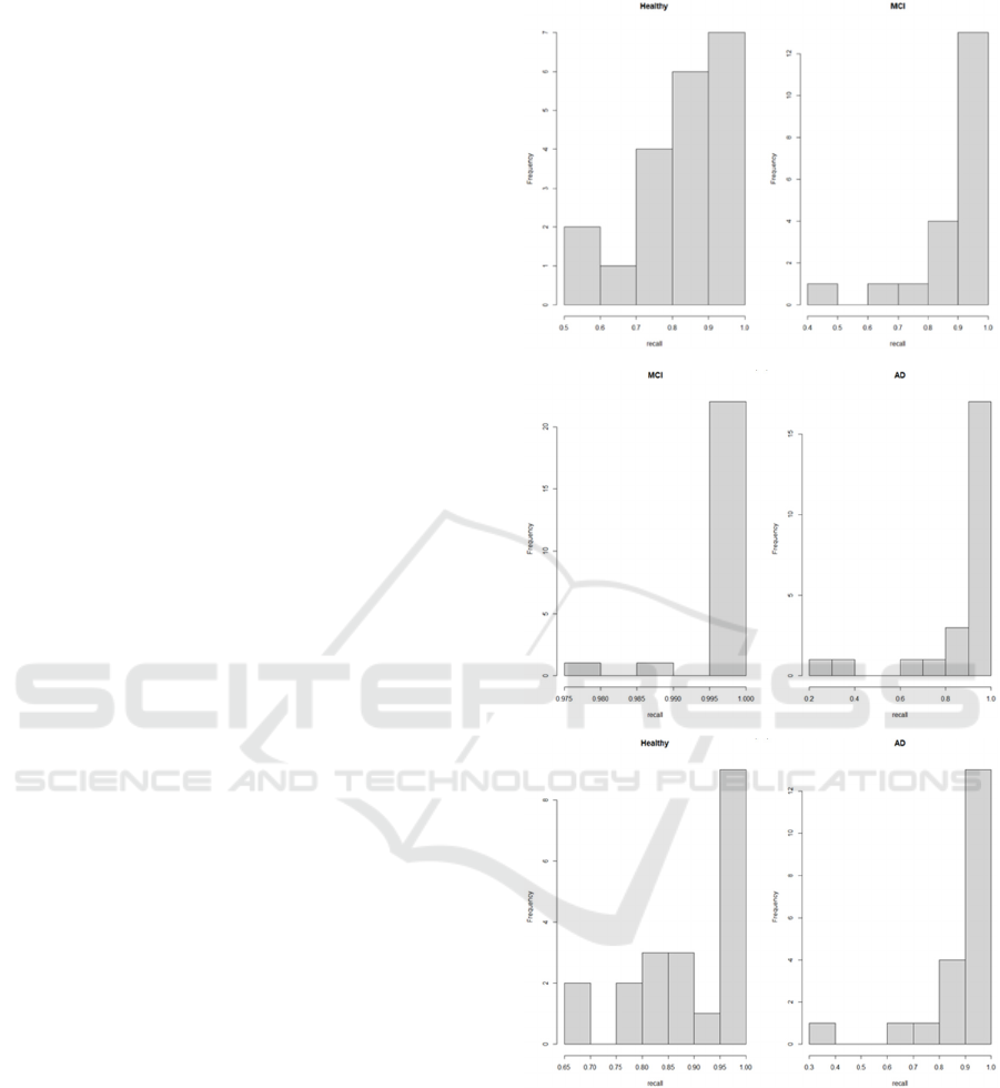
classification, a histogram of the classification recall

per patient is provided (Figure 1). The recall per

patient (TP/TP+FN) shows the percentage of TP vs

FN of the classified segments per patient, and in the

hard voting scheme selected, a recall threshold >=0.6

as selected to suggest a correct patient classification.

As seen in the figures, most of the segments are well

above the 0.6 threshold in all cases. Only in Figure

1a, in the Healthy class, one can see 2 out of the 20

cases where recall is between 0-5 and 0.6, in which

cases we do not conclude with a correct subject

classification.

Table 1 presents the summarised performance

metrics in the testing set regarding the three binary

classification models, with closed eyes and low-pass

filter. In each run, all segments of the 1st class belong

to a single subject of this class that is left out for

testing,

and

the

same

stands

for

the

2nd

class.

The

(a)

(b)

(c)

Figure 1: Distribution of classification recall per patient. a)

Healthy-MCI closed eyes, low band, b) MCI-AD closed

eyes low band, c) Healthy-AD closed eyes low band.

precision and recall metrics are depicted as median

and (1

-3

quantile), corresponding to the

percentages of correctly and falsely classified

segments per subject. The correctly classified

subjects per class are calculated based on recall >0.6

in each run.

Exploring Classiﬁcation in Open and Closed Eyes EEG Data for People with Cognitive Disorders

301

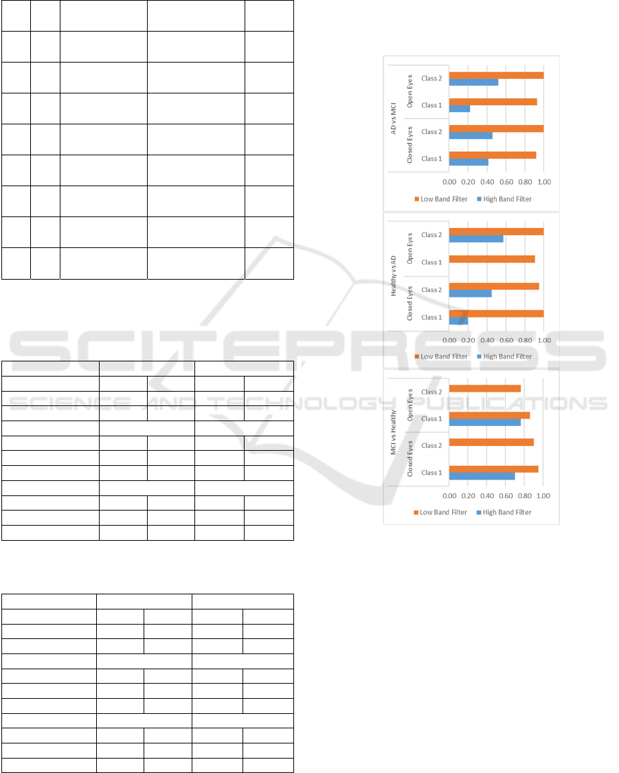
Table 1: Patient Classification performance metrics for the

three binary classification models, using RF classifier and

the majority voting per patient. H stands for Healthy, M for

MCI, A for AD. #C stands for the correctly classified

subjects (correct segments > 60%).

Precision Recall #C

H 0.97

(0.87–1)

0.84

(0.75-0.93)

18 /20

M 0.85

(0.74-0.95)

0.97

(0.86–1)

19 /20

H 0.91

(0.85–1)

0.9

(0.81-0.97)

20/20

A 0.91

(0.84-0.97)

0.93

(0.86–1)

19 /20

M 0.94

(0.88-0.97)

(1-1)

24 /24

A 1

(1–1)

0.93

(0.86-0.97)

22 /24

Table 2: Classification cross-validation results measured in

a range between 0 and 1 in terms of ratio of correctly

classified patients for the AD vs MCI, Health vs AD and

MCI vs Healthy scenario, with all channels.

AD vs MCI Closed Eyes Open Eyes

AD MCI AD MCI

h Band 0.42 0.46 0.22 0.52

Low Band 0.92 1.00 0.93 1.00

Healthy vs AD Closed Eyes Open Eyes

Health AD Health AD

High Band 0.20 0.45 0.00 0.57

Low Band 1.00 0.95 0.90 1.00

MCI vs Health

Closed E

es O

en E

MCI Health MCI Health

High Band 0.70 0.00 0.76 0.00

Low Band 0.95 0.90 0.86 0.76

Table 3: Ratio of patients classified correctly in the three

binary classification scenarios, with selected channels.

AD vs MCI Closed Eyes Open Eyes

AD MCI AD MCI

h Band 0.04 0.58 0.07 0.52

Low Band 0.29 0.96 0.44 1.00

Health

vs AD Closed E

es O

en E

Health AD Health AD

High Band 0.50 0.40 0.00 0.48

Low Band 0.65 0.80 0.71 0.95

MCI vs Health

Closed E

es O

en E

MCI Health MCI Health

h Band 0.65 0.15 0.76 0.00

Low Band 0.90 0.00 1.00 0.00

More detailed results are presented in Table 2 and

Table 3, as regards the different schemes considered.

More specifically, these results show percentages of

correctly classified subjects per class and correspond

to the three binary classification models (based on the

2-stage classifier) and the schemes with 17 vs. 10

channels, open vs closed eyes, and high vs low-

frequency bands.

Figure 2: Classification results (correctly patients classified

ratio) with low / high band filter, with open / closed eyes

and all channels for top) AD vs MCI patients. mid) Healthy

vs AD patients, bottom) MCI vs Healthy patients.

The case with ten selected channels (in the

central-temporal zone) resulted in inferior results,

suggesting that the combined information from all

channels was useful. The case of Healthy vs. AD Low

Band Open Eyes and closed eyes is the only open-eye

case where classification results are quite high.

BIOSIGNALS 2022 - 15th International Conference on Bio-inspired Systems and Signal Processing

302

Figure 3: Classification results (correctly patients classified

ratio) with low/high band filter, with open/closed eyes and

all channels for top) AD vs. MCI patients. mid) Healthy vs.

AD patients, bottom) MCI vs. Healthy patients.

As illustrated in Figure 2, the scheme with the low

band filter and closed eyes works better for every case

in our dataset. In Healthy vs. AD and MCI vs. Healthy

examples, the algorithm returned in total the optimal

accuracy using the low band filter. Figure 3 presents

the correctly classified patients, when selected

channels are used, and performance is overall lower.

Overall, when considering together the results of

low-frequency closed and open eyes, only one AD

and one healthy subject are wrongly classified in both

open and closed eye cases, while one healthy subject

is wrongly classified vs. AD and vs. MCI in open

eyes. All other failures are basically in open eyes,

which is probably a more challenging case and lies in

the inconclusive area, having around 50% of patients’

segments in each class. The combination of both open

and closed eyes in a classification scheme might lead

to interesting results, and even manage to classify into

more subgroups.

Table 4: Summarised performance metrics for the 3-class

classification model. Precision and recall are calculated in

terms of percentages of correctly and falsely classified

segments per subject. Values correspond to median and 1

3d quartiles. The correctly classified patients are depicted

in the #C column.

Precision Recall #C

Healthy 0.96

0.86-1.0

0.85

0.72-0.96

16/20

MCI 0.75

0.69-0.87

0.95-

0.84-1.00

17/20

AD 1.00

0.99-1.00

0.95

0.90-0.98

19/20

In the case of the three-class classification

problem, Table 4 presents similar performance

metrics for the 3-class model in the testing set,

including segments from two subjects in each run.

Metrics include Median (1

-3

quartile) for precision

and recall. Based on recall >0.6 in each run, the last

column shows the correctly classified subjects per

class. Results are slightly poorer in this case than the

binary models as presented in Table 1, especially

regarding the Healthy class. The 3-class model may

require more data for training.

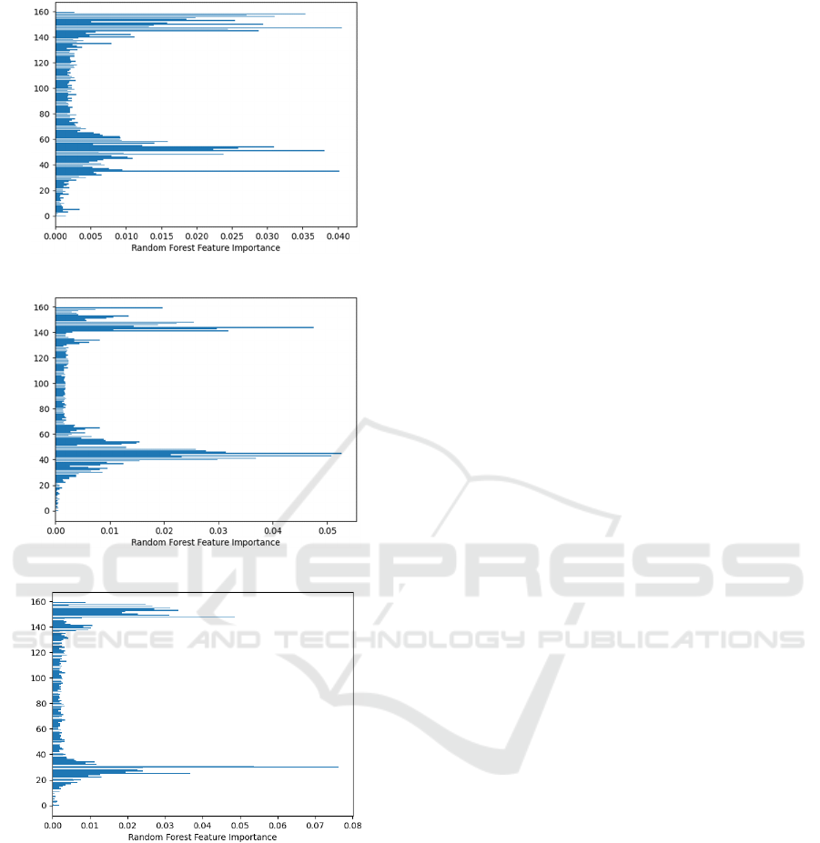
Finally, an important issue that would need to be

addressed is that of exploring feature importance.

KPCA is not directly leading to insights about the

features that lead to best classification, and the

mechanisms behind that, and more sophisticated

methods would be required to illustrate results in

terms of interpretability.

Nevertheless, Figure 4 provides feature

importance, as provided by the RF model, based on

the Gini importance, to illustrate the contribution of

multiple components of the KPCA transform, and

how these differ per classification problem. This

could potentially help in optimising the features

eventually selected in each classification model.

4 CONCLUSIONS

The presented method is based on KPCA for

dimensionality reduction of multichannel segments.

This method has been used before with EEG analysis

(Ye et al, 2018). Considering the classification

results, low band filter returns better accuracy for

both training and test set. Furthermore, the algorithm

works best with AD or MCI vs Healthy patients rather

than AD vs MCI. Compared to the results performed

in the comparative study of (Lehmann et al, 2007), a

rather higher accuracy is achieved. This is probably

because MCI and AD signals share some similarities,

Exploring Classiﬁcation in Open and Closed Eyes EEG Data for People with Cognitive Disorders

303

(a)

(b)

(c)

Figure 4: Feature importance from the Random Forest

model classification results with low band filter, closed

eyes and all channels, for a) Healthy-MCI model, b) for

MCI-AD model, and c) Healthy-AD model. Y-axis

corresponds to 1-160 KPCA components used as features.

and the algorithm faces difficulty to correctly identify

patient data as one of those classes.

While the low frequency closed eyes scheme

seems to produce a better result than open eyes, it is a

matter of further research whether information from

both states would result in more stable and safe

results. Certainly, a larger training dataset and a more

comprehensive evaluation would improve the

credibility of the results. A more thorough finetuning

of the various parameters would also be of value and

would potentially lead to a more optimized outcome.

Furthermore, adding an explainability layer

would help better understand and trust the approach.

Finally, it would be relevant to address the problem

in a continuous space rather than a classification

problem and recognize the problem’s complexity

addressing the different subtypes of the MCI/AD

conditions.

REFERENCES

Amezquita-Sanchez, J. P., Mammone, N., Morabito, F. C.,

Marino, S., & Adeli, H. (2019). A novel methodology

for automated differential diagnosis of mild cognitive

impairment and the Alzheimer’s disease using EEG

signals. Journal of Neuroscience Methods, 322, 88–95.

https://doi.org/10.1016/j.jneumeth.2019.04.013

Awad, M., & Khanna, R. (2015). Support Vector Machines

for Classification. In Efficient Learning Machines (pp.

39–66). Apress. https://doi.org/10.1007/978-1-4302-

5990-9_3

Buegler M, Harms R, Balasa M, Meier IB, Exarchos T, Rai

L, Boyle R, Tort A, Kozori M, Lazarou E, Rampini M,

Cavaliere C, Vlamos P, Tsolaki M, Babiloni C,

Soricelli A, Frisoni G, Sanchez-Valle R, Whelan R,

Merlo-Pich E, Tarnanas I. 2020 Digital biomarker-

based individualized prognosis for people at risk of

Dementia. Alzheimers Dement (Amst). Aug

19;12(1):e12073. doi: 10.1002/dad2.12073. PMID:

32832589; PMCID: PMC7437401.

Dallora, A. L., Eivazzadeh, S., Mendes, E., Berglund, J., &

Anderberg, P. (2017). Machine learning and

microsimulation techniques on the prognosis of

Dementia: A systematic literature review. PLOS ONE,

12(6), e0179804. https://doi.org/10.1371/

journal.pone.0179804

Durongbhan, P., Zhao, Y., Chen, L., Zis, P., De Marco, M.,

Unwin, Z. C., Venneri, A., He, X., Li, S., Zhao, Y.,

Blackburn, D. J., & Sarrigiannis, P. G. (2019). A

Dementia Classification Framework Using Frequency

and Time-Frequency Features Based on EEG Signals.

IEEE Transactions on Neural Systems and

Rehabilitation Engineering, 27(5), 826–835. https://

doi.org/10.1109/TNSRE.2019.2909100

Kim, D., & Kim, K. (2018). Detection of Early Stage

Alzheimer’s Disease using EEG Relative Power with

Deep Neural Network. 2018 40th Annual International

Conference of the IEEE Engineering in Medicine and

Biology Society (EMBC), 352–355. https://doi.org/

10.1109/EMBC.2018.8512231

Kulkarni, N., & Bairagi, V. K. (2014). Diagnosis of

Alzheimer Disease using EEG Signals. International

BIOSIGNALS 2022 - 15th International Conference on Bio-inspired Systems and Signal Processing

304

Journal of Engineering Research & Technology

(IJERT), 3(4).

Kumar, J. S., & Bhuvaneswari, P. (2012). Analysis of

Electroencephalography (EEG) Signals and Its

Categorization–A Study. Procedia Engineering, 38,

2525–2536. https://doi.org/10.1016/

j.proeng.2012.06.298

Lehmann C, Koenig T, Jelic V, Prichep L, et al (2007),

Application and comparison of classification

algorithms for recognition of Alzheimer’s disease in

electrical brain activity (EEG), Journal of Neuroscience

Methods, 161(2), 342-350,ISSN 0165-0270, https://

doi.org/10.1016/j.jneumeth.2006.10.023.

Raz, L., Knoefel, J., & Bhaskar, K. (2016). The

neuropathology and cerebrovascular mechanisms of

Dementia. Journal of Cerebral Blood Flow &

Metabolism, 36(1), 172–186. https://doi.org/10.1038/

jcbfm.2015.164

van der Maaten L., Hinton G. (2008). Visualizing data

using t-SNE. J. Mach. Learn. Res. 9, 2579–2605Wang,

Q. (2012). Kernel Principal Component Analysis and

its Applications in Face Recognition and Active Shape

Models. http://arxiv.org/abs/1207.3538

Ye B, Qiu T, Bai X, Liu P (2018). Research on Recognition

Method of Driving Fatigue State Based on Sample

Entropy and Kernel Principal Component Analysis.

Entropy (Basel). ;20(9):701. doi: 10.3390/e20090701.

PMID: 33265790; PMCID: PMC7513215.

Exploring Classiﬁcation in Open and Closed Eyes EEG Data for People with Cognitive Disorders

305