Interpolated Experience Replay for Continuous Environments

Wenzel Pilar von Pilchau

1 a

, Anthony Stein

2 b

and J

org H

ahner

Organic Computing Group, University of Augsburg, Am Technologiezentrum 8, Augsburg, Germany

Artiﬁcial Intelligence in Agricultural Engineering, University of Hohenheim, Garbenstraße 9, Hohenheim, Germany

Keywords:

Experience Replay, Deep Q-Network, Deep Reinforcement Learning, Interpolation, Machine Learning.

Abstract:

The concept of Experience Replay is a crucial element in Deep Reinforcement Learning algorithms of the

DQN family. The basic approach reuses stored experiences to, amongst other reasons, overcome the problem

of catastrophic forgetting and as a result stabilize learning. However, only experiences that the learner observed

in the past are used for updates. We anticipate that these experiences posses additional valuable information

about the underlying problem that just needs to be extracted in the right way. To achieve this, we present

the Interpolated Experience Replay technique that leverages stored experiences to create new, synthetic ones

by means of interpolation. A previous proposed concept for discrete-state environments is extended to work

in continuous problem spaces. We evaluate our approach on the MountainCar benchmark environment and

demonstrate its promising potential.

1 INTRODUCTION

The combination of neural networks with Reinforce-

ment Learning (RL), also known as Deep RL, has

recently achieved several breakthroughs in the do-

main of Machine Learning. Some prominent exam-

ples range from playing Atari games (Mnih et al.,

2015) over mastering the board game Go on a super-

human level (Silver et al., 2017) to even more com-

plex environments with huge state- and action-spaces

like the video games StarCraft II (Vinyals et al., 2019)

and Dota 2 (Berner et al., 2019).

One well known algorithm in this context is the

so-called Deep Q-Network (DQN) (Mnih et al., 2015)

that replaces the Q-table from the classic Q-Learning

with a neural network. To counteract several prob-

lems that arise here (i.e. correlations of Q-updates

and catastrophic forgetting), the Experience Replay

(ER) was brought back to live, a concept that has

been developed before the wide success of neural net-

works. The ER works as a memory of experienced

situations, similar to the short-term memory of living

individuals, and stores them in a buffer. In the train-

ing phase the learner makes use of them and is able

to increase sample efﬁciency and stabilize the learn-

ing process this way. However, the stored transitions

are only used in the form they have been gathered and

https://orcid.org/0000-0001-9307-855X

https://orcid.org/0000-0002-1808-9758

the possibly existing potential in this collection of ob-

servations of the environment is not further exploited.

As after enough time steps has gone by, the stored

experiences are well distributed over the state space,

and the transitions in the buffer represent knowledge

about the environment that just needs to be extracted

and used in the right way. This is our hypothesis at

least.

The Interpolated Experience Replay (IER) does

exactly that. A ﬁrst study from Pilar von Pilchau et

al. (Pilar von Pilchau et al., 2021) in discrete envi-

ronments with a simplistic and restricted version of

IER showed promising results and justiﬁed a deeper

investigation. Our contribution involves the creation

of synthetic experiences by means of interpolation.

These interpolated experiences are stored in an in-

dividual buffer and mixed in for training. A nearest

neighbour search collects valuable samples from the

real buffer and utilizing the technique of Inverse Dis-

tance Weighting Interpolation (Shepard, 1968) new

synthetic experiences are created. In the early explo-

ration phases, when the learner knows little about the

environment and is building up its knowledge slowly,

the IER shows its potential and results in a reduced

learning time. For evaluation purposes we used the

MountainCar problem and tested several conﬁgura-

tions of IER. Our second contribution is the extension

to deal with continuous state spaces.

von Pilchau, W., Stein, A. and Hähner, J.

Interpolated Experience Replay for Continuous Environments.

DOI: 10.5220/0011326900003332

In Proceedings of the 14th International Joint Conference on Computational Intelligence (IJCCI 2022), pages 237-248

ISBN: 978-989-758-611-8; ISSN: 2184-3236

237

The remainder of the paper is structured as fol-

lows. We give a short introduction of some basic

knowledge like the ER and DQN in Section 2. An

overview of relevant work that has been done in this

area is given in Section 3. A reminder of the basic

functionality of the IER is presented in Section 4 and

followed by our main contribution in Section 5, where

we describe how the IER can be applied for continu-

ous environments. An evaluation on the MountainCar

environment is performed in Section 6. Finally we

conclude the paper with a summary and some ideas

for future work in Section 7.

2 BACKGROUND

In this section we present some background knowl-

edge such as what is an Experience Replay and a short

introduction of the Deep Q-Network.

2.1 Experience Replay

ER is a biological inspired mechanism (McClelland

et al., 1995; O’Neill et al., 2010; Lin, 1992; Lin,

1993) to store experiences and reuse them for train-

ing later on.

An experience is deﬁned as: e

t+1

) where s

denotes the state at

time t, a

the performed action, r

the corresponding

received reward, s

t+1

the follow-up state and d

the reached state was terminal. Each time step t

the agent stores its recent experience in a dataset

= {e

,...,e

}. In a non-episodic/inﬁnite envi-

ronment (and also in an episodic one after a certain

amount of steps) we would run into the problem of

limited storage. To counteract this issue the vanilla

ER is realized as a FiFo buffer. Thus, old experiences

are discarded after reaching the maximum length.

This procedure is repeated over many episodes,

where the end of an episode is deﬁned by a terminal

state. The stored transitions can then be utilized for

training either online or in a speciﬁc training phase.

It is very easy to implement ER in its basic form and

the cost of using it is mainly determined by the stor-

age space needed.

2.2 Deep Q-Learning

The Deep Q-Network was ﬁrst introduced in (Mnih

et al., 2015; Mnih et al., 2013) and is the combina-

tion of classic Q-Learning (Sutton and Barto, 2018;

Watkins and Dayan, 1992) and neural networks. It

approximates the optimal action-value function:

∗

(s,a) = max

bbE



+γr

t+1

+γ

t+2

+.. .|s

= s, a

= a, π



(1)

To enable large continuous state- and action-

spaces and also make use of generalization, the Q-

function is parametrized by a neural network. Equa-

tion (1) displays the maximum sum of rewards r

dis-

counted by γ at each time-step t, that is achievable by

a behaviour policy π = P(a|s), after making an obser-

vation s and taking an action a.

The temporal-difference error δ

is used to per-

form Q-Learning updates at every time step:

= r

+ γmax

Q(s

t+1

) − Q(s

). (2)

Tsitsiklis et al. (Tsitsiklis and Roy, 1997) showed

that a nonlinear function approximator used in combi-

nation with temporal-difference learning, such as Q-

Learning, can lead to unstable learning or even diver-

gence of the Q-function.

As a neural network is a nonlinear function ap-

proximator, there arise several problems:

1. the correlations present in the sequence of obser-

vations,

2. the fact that small updates to Q may signiﬁcantly

change the policy and therefore impact the data

distribution, and

3. the correlations between the action-

values Q(s

) and the target values

r + γ max

Q(s

t+1

) present in the TD-error

shown in (2).

The last point is crucial, because an update to Q

will change the values of both, the action-values as

well as the target values. That could lead to oscilla-

tions or even divergence of the policy. To counter-

act these issues, two concrete actions have been pro-

posed:

1. The use of ER solves, as stated above, the two ﬁrst

points. Training is performed each step on mini-

batches of experiences (s, a, r, s

) ∼ U(D), that are

drawn uniformly at random from the ER.

2. To remove the correlations between the action-

values and the target values, a second neural net-

work is introduced that is basically a copy of the

network used to predict the action-values. This

network is responsible for the computation of the

target values. The target-network is either freezed

for a certain interval C before it is updated again

or “soft” updated by slowly tracking the learned

networks weights utilizing a factor τ. (Mnih et al.,

2015; Lillicrap et al., 2016)

We freeze the target network as presented above

and extend the classic ER with a component to create

synthetic experiences.

NCTA 2022 - 14th International Conference on Neural Computation Theory and Applications

238

3 RELATED WORK

The classical ER, introduced in Section 2.1, has been

improved in many further publications. One promi-

nent improvement is the so called Prioritized Experi-

ence Replay (Schaul et al., 2015) which replaces the

uniform sampling with a weighted sampling in favour

of experience samples that might inﬂuence the learn-

ing process most. This modiﬁcation of the distribu-

tion in the replay induces bias, and to account for

this, importance-sampling has to be used. The au-

thors show that a prioritized sampling leads to great

success. This extension of the ER also changes the de-

fault distribution, but uses real transitions and there-

fore has a different focus.

Another extension of the classic ER is the

so-called Hindsight Experience Replay (HER)

(Andrychowicz and others, 2017). The authors

investigated multi-objective RL problems and used

state-action-trajectories alongside a given goal as

experiences to store in their HER. In complex envi-

ronments the agent was not able to understand what

goal it is intended to reach and therefore was not suc-

cessful. To assist the learner, synthetic experiences

were introduced and saved together with the real

ones. Such an experience replaced the goal with the

last state in the trajectory. This technique helped the

learner to understand what a goal is and subsequently

to reach the environment-given goals. In contrast to

our approach HER uses trajectories as experiences

and solves multi-objective environments, also no

interpolation is used to create synthetic experiences.

The authors of (Rolnick et al., 2018) presented

CLEAR, a replay-based method that greatly reduced

catastrophic forgetting in multi-task RL problems.

Off-policy learning and behavioural cloning from re-

play is used to enhance stability. On-policy learning

guarantees a preserved plasticity. In contrast to our

approach CLEAR does not use any form of synthetic

experiences and is designed for actor-critic algorithms

instead of DQN.

In (Hamid, 2014) the author investigates the ef-

fect of reappearing context informations. Two differ-

ent learners are used to learn the relation of states and

actions and reoccurring sequences into a data stream.

The data comes in three subsequences called context

and the ﬁrst and the last context are the same while

the middle context differ. The author could show that

the information that was learned in context 1 can be

reused in context 3 even after confronted with a com-

pletely new context in between. The approaches ex-

tracts temporal information from previously observed

experiences to avoid catastrophic forgetting. IER uses

collected experiences to create completely new expe-

riences and therefore differ from this approach.

Sander uses interpolation to create synthetic ex-

periences for a replay buffer (Sander, 2021). In con-

trast to our approach, the used buffer is completely

ﬁlled with interpolated experiences and the synthetic

samples are generated from the corresponding neigh-

bourhood with mixup. The interpolation is performed

in every step and until the algorithm stops, while we

start with a high number of interpolations and end up

with very little or even no interpolations as we reach

convergence. The approach from Sander is located,

evaluated and motivated in the control task domain.

This work draws on the methods proposed in e.g.

(Stein et al., 2017; Stein et al., 2018). The authors

used interpolation in combination with an XCS clas-

siﬁer system to speed up learning in single-step prob-

lems by means of using previous experiences as sam-

pling points for interpolation. Our approach focuses

on a DQN as learning component and more impor-

tantly sequential decision problems.

4 INTERPOLATED EXPERIENCE

REPLAY BASICS

This work builds upon the ﬁndings of (Pilar von

Pilchau et al., 2020; Pilar von Pilchau, 2019; Pilar von

Pilchau et al., 2021). We give a short recap of the ba-

sics of the Interpolated Experience Replay (IER) in

the following chapter.

The IER makes use of the architectural concept

of the Interpolation Component (IC) from Stein et al.

(Stein et al., 2017). The actual IER consists of two

separated parts that share a maximum size: (1) The

real experience buffer and (2) the buffer for interpo-

lated experiences (cf. Fig. 1). The original synthetic

experience buffers size is restricted by the amount

of stored real samples and therefore decreasing over

time. If the buffer runs full with real experiences then

there is no space left for synthetic ones. This decision

comes from the expectation that an experience cre-

ated directly from the environment is exact, where in

contrast an interpolated one suffers from uncertainty.

Anyhow, to have the possibility to reserve a small

space for synthetic experiences even if the buffer is

full with real samples, there is a minimum size of the

synthetic buffer introduced s

syn min

. Following this,

the maximum size of the IER is the real buffers max-

imum size plus the synthetic buffers minimum size.

We denote the size of the IER as s

ier

, the size of the

real valued buffer as s

and the size of the synthetic

buffer as s

syn

To create synthetic experiences the stored real ex-

perience samples are used as sampling points for in-

Interpolated Experience Replay for Continuous Environments

239

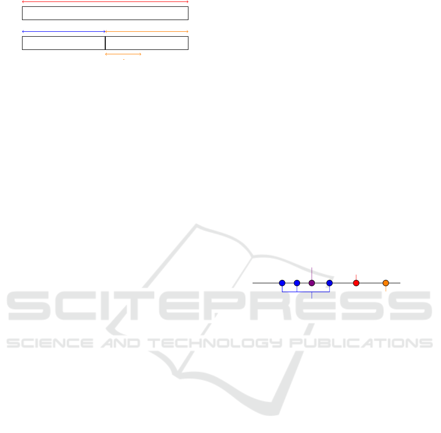
Interpolated Experience Replay

real experiences synthetic experiences

ier

syn

syn min

Figure 1: Intuition of Interpolated Experience Replay mem-

ory.

terpolation. After every step a query point is drawn

from the state space using a query function. Different

query functions were evaluated in (Pilar von Pilchau

et al., 2021), such as drawing at random and different

variations of drawing from the distribution created by

the policy. This query point is then used to gather

all relevant sampling points via a nearest-neighbour

search. A simple averaging of the reward together

with a set of all observed follow-up states is then used

to create a bunch of synthetic experiences for the dis-

crete environment.

For training, the agent samples at random from

the combined buffer of both experiences. The IER is

ﬂooded with synthetic experiences in early steps and

assists the learner when it knows little about the en-

vironment. Following this approach it was possible

to reduce the exploration phase in combination with

increased efﬁciency and as a result the agent was able

to converge faster.

5 INTERPOLATED EXPERIENCE

REPLAY FOR CONTINUOUS

ENVIRONMENTS

Our approach extends the IER for discrete and non-

deterministic environments (Pilar von Pilchau et al.,

2021) with the ability to interpolate follow-up states

instead of a simple average calculation of just the re-

wards. This makes it possible to use the IER in con-

tinuous environments. In this section we present the

novel functionalities.

Most importantly, it was necessary to allow it for

continuous environments. To achieve this, we needed

to solve the problem of the unknown follow-up state

of a synthetic experience, which is an important com-

ponent. Uncertainty here is expected to harm the

learning process in a way that would make the whole

approach unusable, because the Q-update relies on

predictions of these. In this section, we present a so-

lution for this issue.

5.1 Interpolation of the Follow-up

States

A straightforward solution, following the reward av-

eraging approach of (Pilar von Pilchau et al., 2021),

would be an interpolation of the follow-up state based

on the detected nearest-neighbours. In a very simple

environment where the agent can only move left or

right the state is represented by a position on a line.

Imagine the situation when the query point equals the

biggest yet discovered position to the right. Conse-

quently all sampling points have to be on the left of

this point. An interpolation of the follow-up state for

the action “move right” would result in a position that

is also located to the left of the query point but in fact

should be to the right. This effect (illustrated in Fig. 2)

would create a synthetic experience that is mislead-

ing as it assigns a movement in the wrong direction

to the move to the right action. In fact, the expected

behaviour that we want would be considered as ex-

trapolation which is known to be inaccurate or at least

suffers from uncertainty.

query point

true follow-up state

interpolated follow-up state

sampling points

Figure 2: Illustration of how interpolation of follow-up

states can create misleading results.

As a consequence, we developed a new approach

of interpolating the follow-up state. As the state-

transition of all observed experiences directly corre-

lates with the corresponding start state we decided to

interpolate the state-transition instead. In the above

mentioned example, all state-transitions (calculated

as δ

= s

t+1

−s

) of the discovered nearest-neighbours

are used as sampling points and an interpolated state-

transition is created and added to the sampling point.

As can be seen in Fig. 3 the interpolated follow-up

state equals the real follow-up state in the simple ex-

ample. This effect also holds for more complex states,

like a combination of position and velocity, as long

as s

t+1

is directly dependant from the corresponding

state s

. In more complex environments the interpola-

tion might not be exactly the same as the real value but

indeed suffers from reduced uncertainty compared to

the interpolation of the follow-up state directly. Fol-

lowing this approach we are still able to use interpo-

lation techniques for a (potential) extrapolation task.

NCTA 2022 - 14th International Conference on Neural Computation Theory and Applications

240

query point

true/interpolated

follow-up state

sampling points

true/interpolated

state-tranistion

Figure 3: Illustration of the interpolation of state-transitions

to calculate a stable approximation of the follow-up state.

5.2 Interpolation Technique

The equally weighted average interpolation used in

(Pilar von Pilchau et al., 2021) was introduced for a

ﬁrst analysis of the idea and more complex environ-

ments require more complex interpolation techniques.

Thus, we decided to use Inverse Distance Weight-

ing Interpolation (IDW) (Shepard, 1968) for our ap-

proach.

IDW strives to create an interpolation using a

weighted average, where sampling points that are lo-

cated in closer distance to the query point have big-

ger impact than sampling points located farther away.

IDW is deﬁned as follows:

u(~x) =







∑

i=1

(

x)u

∑

i=1

(~x)

, ifd(~x,~x

) 6= 0 for all i,

ifd(~x,~x

) = 0 for some i,

(3)

with

(~x) =

d(~x,~x

)

. (4)

The interpolation function tries to ﬁnd an inter-

polated value u at a given point ~x based on sampling

points u

= u(~x

)fori = 1, 2, . ..,N. To increase the im-

pact of closer values a weight w

is used that includes

a distance metric d together with a variable p called

the power parameter controlling the impact of u

In our approach, we use experiences e

i+1

) as samples u

. A query point ~x =

= (s

) is received via a query function and the

euclidean distance of the states s

and s

is used as

distance metric d. Furthermore the amount of sam-

pling points is restricted by the action a

and a nearest

neighbour search so that only experiences that meet

the following condition are included:

d(~x

,~x

) ≤ nn

thresh

∧ a

== a

, (5)

where nn

thresh

deﬁnes the maximum search radius.

The interpolation only occurs for the values of r

, s

i+1

and d

, resulting in the corresponding interpolations

r(~x), s

t+1

(~x) and d(~x). We can then create an interpo-

lated experience:



,r(~x), s

t+1

(~x),d(~x)



(6)

5.3 Synthetic Buffer Size

To original concept of a shared maximum size as pre-

sented in Section 4 is a quite simple approach and

lacks the ability of ﬁne-tuning. As a consequence, we

introduce two new functionalities: (1) an exploration

mode and (2) the parameter β. The former deﬁnes a

minimum size of the synthetic buffer msexpl in rela-

tion of the actual decaying exploration rate ε and the

allowed maximum size s

syn max

msexpl

= ε

∗ s

syn max

. (7)

The parameter β allows a ﬁner tuning of the mini-

mal size of the synthetic buffer in later stages. Thus, β

inﬂuences the minimum size of the buffer s

syn min

(cf.

Section 4). Another minimum size msbeta is then de-

ﬁned as follows:

msbeta

= bs

syn min

∗ β

c, (8)

with

= max



init

−



init

∗ i





. (9)

init

is the initial value that is assigned to β and

1 was found as a good value here. Furthermore, β

decreases after every time step i (an episode in our

approach) until it reaches 0 in time step M.

Following (7) and (8) we can update the minimal

size of the synthetic buffer s

syn min

for every episode

as follows:

syn min

= max



msexpl

,msbeta

] (10)

Fig. 4 gives a graphical intuition of how the mini-

mum size of the synthetic buffer is determined.

size

syn max

syn min

msbeta

msexpl

Figure 4: Intuition of the synthetic buffers minimal size.

Interpolated Experience Replay for Continuous Environments

241

5.4 Distribution Sampling

An evaluation of different query functions in (Pi-

lar von Pilchau et al., 2021) revealed that the IER

beneﬁts from a sampling method that follows the dis-

tribution that is created by the policy. We can ﬁnd

an off policy equivalent of this distribution in the real

experience buffer as it was created by the policy. In

discrete environments, it was enough to draw an ex-

perience out of the real valued buffer and use the re-

ceived state-action pair as query point. This is no

longer reasonable for continuous environments, be-

cause we are faced with a much bigger state space and

want to explore it instead of just interpolate points for

which we already know the exact corresponding re-

ward and follow-up state. We needed to adapt this

method to work again and to achieve this, we decided

to draw the query point in a radius r

around the state

received from the drawn real example. To simplify

this parameter for multidimensional state spaces, we

deﬁned it as follows: 0 ≤ r

≤ 1. As we know the

maximum value of each dimension, we are now able

to determine a corresponding radius for each dimen-

sion:

= r

∗ S

max

∀ d ∈ S

dim

, (11)

with S

dim

being the dimensionality of the state

space. If the state space is deﬁned as inﬁnite for one or

more dimensions we can track the maximum discov-

ered value for the appropriate dimension(s) and use

this value(s) instead. To follow an on policy variation

of the distribution we always use the state-action pair

that was recently created by the policy instead of sam-

pling from the buffer. We call the former method Pol-

icy Distribution (PD) and the latter Last State (LS).

To follow the policy distribution even closer we can

choose the action of x

according to the actual pol-

icy, otherwise we perform an interpolation for every

action from the action space.

The associated pseudocode that summarizes the

procedure is depicted in Algorithm 1.

5.5 Performant Nearest Neighbour

A straightforward approach of ﬁnding all relevant

neighbours that satisfy the ﬁrst part of (5) would be

an exhaustive search in the real buffer. As this would

result in a computation time of O(N) we were in the

need of ﬁnding a more efﬁcient solution. We decided

to go with the ball-tree structure (Omohundro, 1989)

that reduces the computation time to O(logN).

As this technique is designed for a static dataset

we are forced to rebuild the tree in a ﬁxed interval

Algorithm 1: IER for continuous environments.

Initialize D

real

and D

inter

Initialize β, t

βmax

, ε and nn

thresh

Initialize s

syn max

, s

syn min

, IER

size

and t

max

dec

βmax

while t not t

max

while s is not TERMINAL do

Store experience e in D

if |D

real

| ≥ c

start inter

∧ s

syn min

> 0 then

Get x

= (s

)

from Query Function

Get



|d(~x

,~x

) ≤ nn

thresh

∧ a

= a



from D

real

Store results in D

match

Compute ~x from IDW (x

match

)

Create e

= (s

,r(~x), s

t+1

(~x),t(~x))

Store e

in D

inter

sp = max[s

syn min

,IER

size

− |D

real

while |D

inter

| > min[sp,s

syn

max

] do

Remove e from D

inter

sp = max[s

syn min

,IER

size

− |D

real

end while

end if

end while

β ← β − β

dec

Update ε

syn min

← max[mseplx

,msbeta

]

end while

rebalance

, resulting in a ﬁxed set of searchable expe-

riences until the next rebuild appears. We found this

trade-off to be acceptable as the amount of reduced

time needed for searching outweighs the effect of per-

forming nn search on outdated data, especially as all

data will still be inserted into the set of searchable ex-

periences with a maximum delay of nn

rebalance

6 EVALUATION

In this section, we introduce the experimental setup

and afterwards report on the obtained results followed

by a discussion.

6.1 Experimental Setup

6.1.1 Environment

We evaluated our IER approach on the prominent

benchmark MountainCar-v0 environment from Ope-

nAI Gym (Brockman and others, 2016). In this prob-

lem an agent, the mountain car, starts in between two

hills and has to reach the top of the right hill. The

NCTA 2022 - 14th International Conference on Neural Computation Theory and Applications

242

action space covers three actions: (1) move to the

left, (2) move to the right and (3) do nothing. As the

power of the car on its own is not enough to climb the

hill, it has to go as high as possible on one side and

use the gathered speed to reach height on the other

side. By exploiting this effect the agent is able to ﬁ-

nally reach the goal on the right hill. A state is con-

sequently formed out of two parts, (1) the position

and (2) the velocity. An episode is over if the agent

reaches the goal or a maximum time limit of 200 steps

is exceeded. Fig. 5 illustrates the environment.

Car

Goal

state: [x, v]

Figure 5: A graphical illustration of the MountainCar-v0

environment.

In the version from OpenAI Gym the agent re-

ceives a reward of -1 in every step until it reaches the

goal and receives a reward of 0 instead. To make the

reward function interpolatable, we changed it to the

following continuous version found by

r(s

t+1

) =







200 − t ifs

t+1

is terminal,

100 ∗



E(s

t+1

) − E(s

)



else,

(12)

where

E(s) =

sin(3 ∗ x(s))

400

v(s)

, (13)

with x(s) being the position and v(s) the velocity

of the state s. This reward function takes the mechan-

ical energy (kinetic + potential energy) into account,

gives bigger rewards if the agent builds up speed and

height and encourages faster solutions.

6.1.2 Hyperparameter

Preliminary experiments revealed a stable hyperpa-

rameter conﬁguration as given in Table 1.

6.1.3 Experiments

As baseline we used a DQN with vanilla ER and com-

pared it with several conﬁgurations of the IER. All ex-

periments were repeated 20 times with random seeds

and the average return over 100 episodes was mea-

sured alongside the standard deviation. The Moun-

tainCar problem is considered to be solved if theagent

receives a minimum return of -110 over 100 episodes

https://github.com/msachin93/RL/blob/master/

MountainCar/mountain car.py

Table 1: Overview of hyperparameters applied for the

MountainCar-v0 experiment.

Parameter Value

learning rate α 0.00015

discount factor γ 0.95

epsilon start 1

epsilon min 0

target update frequency C 5

real buffer size s

50,000

start learning at size 2,000

minibatch size 32

start interpolation c

start inter

100

double True

duelling True

hidden layer [50, 200, 400]

nn search space nn

thresh

0,005

rebuild interval nn

rebuild

2,000

query radius r

0,05

beta start β

init

reduce beta until M 1,500

max size of syn buffer s

syn max

50,000

min size of syn buffer s

syn min

20,000

measured by the original reward function. For the

sake of comparability and to make the result inter-

pretable in relation to this criteria, we print the orig-

inal reward functions results, even if we internally

used the reward function presented above. A suc-

cessful completion of the environment indicates faster

learning. The investigated conﬁgurations differ in

the Query Method (Policy Distribution (PD) and Last

State (LS) cf. Section 5.4), and the usage of Explo-

ration Mode (EM) for the calculation of s

syn min

(cf.

Section 5.3) and on policy action selection (cf. Sec-

tion 5.4). A list of all conducted experiments can be

found in Table 2.

Table 2: An overview of all 8 conducted experiments and

the corresponding conﬁgurations.

ID PD/LS EM on policy

PD PD

PD op PD X

PD EM PD X

PD EM op PD X X

LS LS

LS op LS X

LS EM LS X

LS EM op LS X X

Each conﬁguration was tested against the baseline

and the differences have been assessed for statistical

signiﬁcance. A visual inspection of QQ-plots in con-

junction with the Shapiro-Wilk (SW) test revealed that

no normal distribution can be assumed. Since this cri-

terion could not be conﬁrmed for any of the exper-

Interpolated Experience Replay for Continuous Environments

243

Table 3: All conducted experiments and the corresponding

statistical results of the hypothesis tests. In the second col-

umn t

solved

represents the time step when the conﬁguration

solved the problem on average. The next column shows

the standard deviation in episodes over all repetitions for

the time of solving the problem. A lower value of t

solved

indicates faster learning and signiﬁcantly better results are

displayed as underlined entries.

ID t

solved

±1SD SW MWU

baseline 1751 ±551 0.0

PD 1640 ±773 0.0 0.0924

PD op 1403 ±661 0.0 1.8467e-80

PD EM 1727 ±814 0.0 0.0106

PD EM op

1834 ±864 0.0 2.9039e-07

LS 1479 ±697 0.0 0.0002

LS op 1618 ±762 0.0 0.4809

LS EM 1665 ±784 0.0 0.0003

LS EM op 1619 ±763 0.0 2.1847e-11

iments, we chose the Mann-Whitney-U (MWU) test.

All corresponding p-values for the hypothesis test can

be found in Table 3, together with the average episode

of solving the problem alongside the corresponding

standard deviation (±1SD).

6.2 Experimental Results

The results of all experiments are depicted in Fig. 6.

The dotted brown line at -110 indicates the moment

when the problem is considered as solved in the liter-

ature (Sutton and Barto, 2018). The baseline is repre-

sented by the red dashed and the best conﬁguration by

the blue dash-dotted line. We can see that the baseline

steeply increases until about episode 400, then ﬂattens

and drops at around episode 500 to recover slowly.

Most IER conﬁgurations, although also ﬂattening, do

not drop and additionally do not ﬂatten the same level

as the baseline does, except LS op. All conﬁgurations

(except PD EM op) solve the problem faster than the

baseline and stay above the baselines curve beginning

at around episode 400.

Figure 6: All conducted experiments.

As the differences between the IER conﬁgurations

are not that big, it is difﬁcult to distinguish them and

therefore we provide a reduced view of just the base-

line and the best conﬁguration in Fig. 7. Here we can

observe the same behaviour as described above. The

PD op conﬁguration crosses the dotted line at episode

1403 whereas the baseline needs another 348 more

episodes. In this reduced visualization we can clearly

observe that both curves equal each other in the be-

ginning and then, starting at around episode 300, the

IER conﬁguration remains above the baseline.

Fig. 8, Fig. 9 and Fig. 10 show the errors of the re-

ward, the next step and the terminal tag interpolation

averaged over all repetitions. The blue points repre-

sent the maximum error that occurred in an episode

and the red points depict the average error in an

episode. The ﬁrst occurring errors can be spotted at

episode 100 which is because interpolation starts not

before this point in time (cf. Section 6.1.2). The max-

imum error of the interpolated error starts to grow,

beginning at around episode 200, this is caused by the

ﬁrst time that the problem is solved, here a reward

up to 200 is earned. As an interpolated experience

lacks the value for elapsed time steps, that is used in

our custom reward function, we determine a reward of

200 for every experience that solves the environment.

In fact, the reward, and therefore also the interpolated

reward ranges from 0 to 200, dependant of the time

step and, following that the speed and height of the

query point. We can see that the calculated max er-

rors range in between 40 and 100 for the whole run.

The average error on the other side stays below 5 the

whole time. If we take a look at the error of the in-

terpolated follow-up states, we can see that the maxi-

mum error decreases over time and never grows over

a value of 0.012. The average error, also decreasing,

never exceeds a value of 0.002. The terminal tag is

encoded as a boolean and can therefore be either one

or zero. We can observe that in the beginning the max

Figure 7: LS op conﬁguration in comparison with the base-

line.

NCTA 2022 - 14th International Conference on Neural Computation Theory and Applications

244

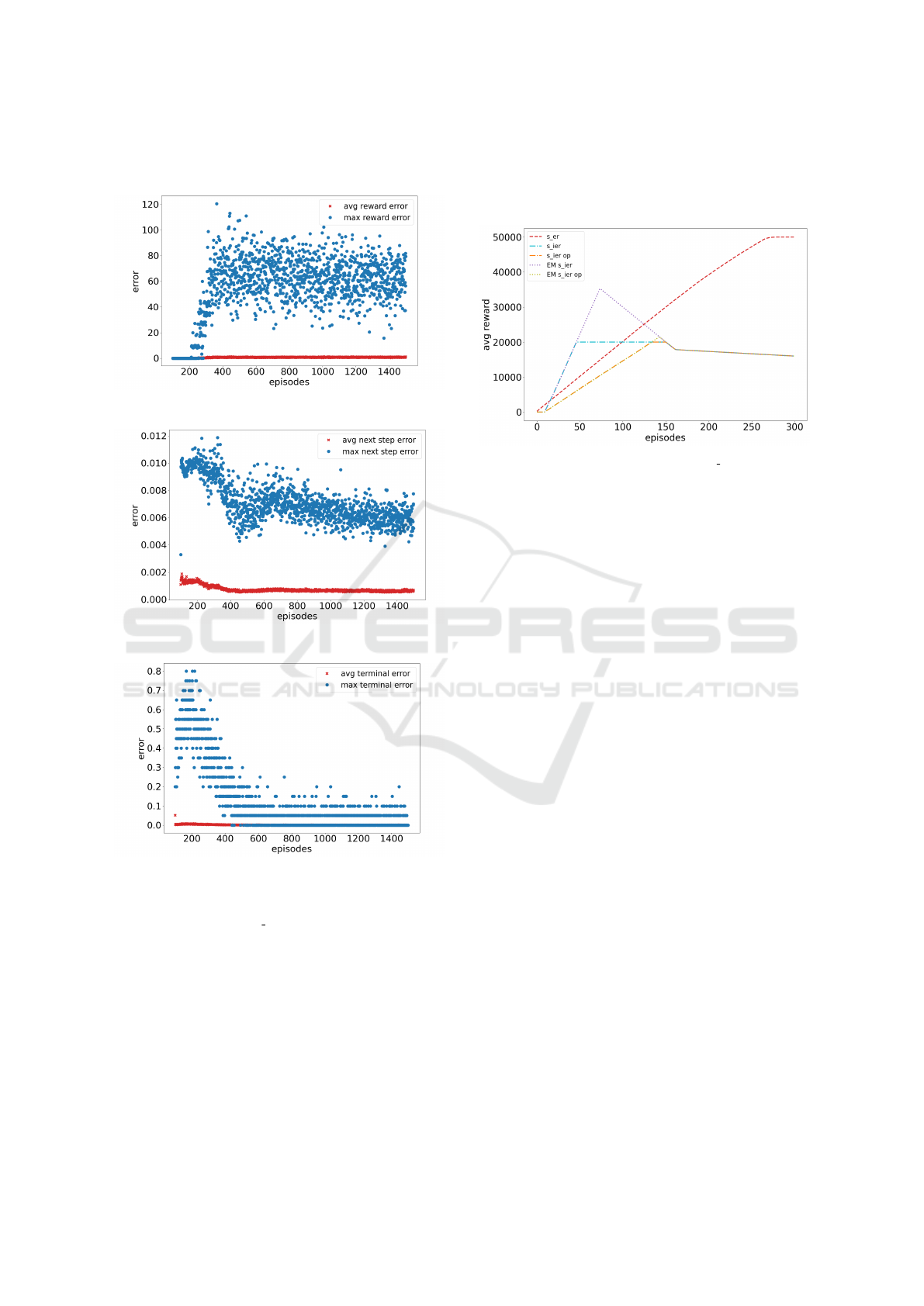
error over all repetitions is close to the maximum but

decreases to around 0.1 in the end.

Figure 8: The interpolation error of the rewards.

Figure 9: The interpolation error of the next steps.

Figure 10: The interpolation error of the terminal tag.

A visualization of the different investigated meth-

ods for calculating s

syn min

is given in Fig. 11. All

modes used beta with the values given in Table 1, the

dotted lines additionally made use of the exploration

mode. The red dashed line represents the size of the

real valued buffer. It can be observed that the usage

of the exploration mode allows a larger size of the

synthetic buffer in the beginning, when exploration is

active, and then meets the decreasing min size set by

beta. The curves for the on policy mode is slightly

shifted to the right caused by lesser interpolations

(one interpolation at maximum per step). We chose to

show not the whole length of the experiments to focus

on the important part that is located in the beginning.

All s

ier

curves decrease to 0 at episode 1500 as deter-

mined by the hyperparameter set in Section 6.1.2.

Figure 11: An intuition of s

syn min

6.3 Interpretation

The results from Fig. 6 and Table 3 show that the ma-

jority of the tested conﬁgurations perform better than

the baseline and can reach the deﬁned goal in less

episodes. This shows that our approach works and

can assist learners in early learning phases.

The exploration mode functionality did not turn

out to be helpful. It performed less effective than

the conﬁguration with just the β determined min size.

Even if this functionality did not prove to be helpful

here, it remains an important adjusting mechanism for

other environments. Fig. 11 shows that the effect was

not too large in our experiments which also is due to

a short exploration time.

A clear statement about the effect of the on policy

action selection mode turns out to be not that obvious.

The best conﬁguration makes use of it and performs

better than just the PD querying, but that does not

hold for the LS method and in combination with EM

it seems to perform better than just the usage of EM

for both. The difference between PD and LS might

result from the fact that we already try to follow the

policy close enough in the case of LS and pushing the

interpolations even more into that direction harms the

approach rather than helping. On the other hand the

PD method follows the policy to a certain extend, but

remains with some degrees of freedom which is then

limited by the on policy action selection in a way that

appears beneﬁcial. The positive effect in combination

with EM is expected to be due to the decreased num-

ber of interpolations that occur resulting in a maxi-

mum size of the synthetic buffer that almost equals

the conﬁgurations without EM (see Fig. 11).

A closer look at Fig. 7 reveals that the PD op con-

ﬁguration performs very well compared to the base-

Interpolated Experience Replay for Continuous Environments

245

line. Not only is the problem solved considerably

faster, but the agent performs also signiﬁcantly bet-

ter after episode 300.

Considering the interpolation errors from Fig. 8,

Fig. 9 and Fig. 10, we can conclude the following:

The error of the interpolated follow-up states is quite

small and even decreases over time. This indicates

a sufﬁcient accuracy here and also that the interpo-

lation beneﬁts from the exploration of the problem

space. The reward error on the other hand seems quite

high, even if it stays below 50%. One cause (as noted

above) lies in the comparison of the different reward

functions. As a query point does not include a time

step and the internal reward function does require one,

we set the t for the interpolation to zero. This has the

effect that the calculated expected reward that we use

then for the determination of the accuracy is always

200. As it is impossible to reach the goal at time step

0 any interpolation will be assigned an error greater

0. This results in an overestimation of the reward er-

rors for reaching the goal but on the other hand still

gives us a good indication of the quality of our inter-

polations. The other point comes from the fact that

we average the reward of neighbouring experiences,

causing interpolations of transitions slightly to the left

of the goal to be overestimated. However, this effect

turns out to be beneﬁcial, because it increases the area

in which experiences are rewarded and therefore helps

the learner to understand that being near the goal is es-

sential for solving the environment. Another insight is

that the average error is way smaller, which indicates

that most of the interpolations are quite accurate. The

error of the terminal tag seems quite high in the begin-

ning of the training, but this can be explained by the

fact that the agent (in early phases) terminates because

of the time limit which is dependant of the time step.

As t is set to zero for the interpolation (see above) an

interpolated experience that copies such a behaviour

is always punished by the error calculation. Over time

the error decreases and in the end we can achieve a

maximum error at around 0.1 which equals errors of

the terminal tag in 2 of the 20 repetitions. Overall the

mean error is around zero the whole time indicating a

good interpolation of the terminal tag in general.

7 SUMMARY AND FUTURE

WORK

We presented an extension of the IER method, so far

proposed for discrete environments only. Our con-

tribution encompasses the interpolation of follow-up

states which makes the IER ready for continuous state

spaces. We presented a solution to interpolate state-

transitions instead of follow-up states directly. This

procedure solves the occurrence of inaccurate results

when an interpolation technique is used for an ex-

trapolation task. A small example shows when this

happens and why this is reasonable. We introduced

several methods to offer the ability of ﬁne-tuning the

synthetic buffers size.

An evaluation on the MountainCar environment

revealed that the approach works. We conducted nu-

merous experiments which the majority of performed

better than the baseline consisting of a DQN with

vanilla ER applied. Our best conﬁguration was able

to solve the problem about 15% faster (episodes).

The introduced exploration mode mechanic did not

turn out to be useful, but nevertheless remain a useful

mechanism for future investigations.

The presented approach can be used for other en-

vironments as well, if the interpolation of reward,

follow-up state and terminal tag is sufﬁciently accu-

rate then it is expected that the results resemble those

presented in this paper. The interpolation techniques

used here are still relatively simple and there are more

complex ones (i.e. radial basis function interpola-

tion (Wright, 2003)) that should be able to interpolate

more difﬁcult tasks with bigger state spaces.

We will test the IER for continuous environments

on other problems to ratify the obtained results. Such

will range from CartPole to even more complex prob-

lems like robotic tasks. Even image inputs can be in-

vestigated with the presented approach, an interpola-

tion of the feature outputs of the convolutional part of

the neural network seems like an idea that should be

investigated further. Also other algorithms that uti-

lize an ER will be evaluated with IER. An interesting

example is soft actor-critic (Haarnoja et al., 2018).

Another interesting ﬁeld, that furthermore bears

some similarities with the examined area, is the re-

search topic of model-based RL. These kind of algo-

rithms create a model to build up knowledge of the

underlying problem which can then be utilized to train

a policy. We locate our approach in between model-

based and model-free RL methods, as we do not build

a complete model but do something similar in com-

bination with model-free RL learners. However, an

investigation of the IER approach from the view of

model-based RL methods could be beneﬁcial.

REFERENCES

Andrychowicz and others (2017). Hindsight Experience

Replay. In Advances in Neural Information Process-

ing Systems 30, pages 5048–5058. Curran Associates,

Inc.

NCTA 2022 - 14th International Conference on Neural Computation Theory and Applications

246

Berner, C., Brockman, G., Chan, B., Cheung, V., Debiak,

P., Dennison, C., Farhi, D., Fischer, Q., Hashme, S.,

Hesse, C., J

ozefowicz, R., Gray, S., Olsson, C., Pa-

chocki, J., Petrov, M., Pinto, H. P. d. O., Raiman,

J., Salimans, T., Schlatter, J., Schneider, J., Sidor,

S., Sutskever, I., Tang, J., Wolski, F., and Zhang,

S. (2019). Dota 2 with Large Scale Deep Rein-

forcement Learning. CoRR, abs/1912.06680. arXiv:

1912.06680.

Brockman, G. and others (2016). OpenAI Gym. eprint:

arXiv:1606.01540.

Haarnoja, T., Zhou, A., Hartikainen, K., Tucker, G., Ha, S.,

Tan, J., Kumar, V., Zhu, H., Gupta, A., Abbeel, P.,

and Levine, S. (2018). Soft Actor-Critic Algorithms

and Applications. CoRR, abs/1812.05905. arXiv:

1812.05905.

Hamid, O. H. (2014). The role of temporal statistics in the

transfer of experience in context-dependent reinforce-

ment learning. In 2014 14th International Conference

on Hybrid Intelligent Systems, pages 123–128.

Lillicrap, T. P., Hunt, J. J., Pritzel, A., Heess, N., Erez, T.,

Tassa, Y., Silver, D., and Wierstra, D. (2016). Con-

tinuous control with deep reinforcement learning. In

Bengio, Y. and LeCun, Y., editors, 4th International

Conference on Learning Representations, ICLR 2016,

San Juan, Puerto Rico, May 2-4, 2016, Conference

Track Proceedings.

Lin, L.-J. (1992). Self-improving reactive agents based on

reinforcement learning, planning and teaching. Ma-

chine Learning, 8(3):293–321.

Lin, L.-J. (1993). Reinforcement learning for robots us-

ing neural networks. Technical report, CARNEGIE-

MELLON UNIV PITTSBURGH PA SCHOOL OF

COMPUTER SCIENCE.

McClelland, J. L., McNaughton, B. L., and O’Reilly, R. C.

(1995). Why there are complementary learning sys-

tems in the hippocampus and neocortex: insights

from the successes and failures of connectionist mod-

els of learning and memory. Psychological review,

102(3):419. Publisher: American Psychological As-

sociation.

Mnih, V., Kavukcuoglu, K., Silver, D., Graves, A.,

Antonoglou, I., Wierstra, D., and Riedmiller, M. A.

(2013). Playing Atari with Deep Reinforcement

Learning. CoRR, abs/1312.5602.

Mnih, V., Kavukcuoglu, K., Silver, D., Rusu, A. A.,

Veness, J., Bellemare, M. G., Graves, A., Ried-

miller, M., Fidjeland, A. K., Ostrovski, G., and others

(2015). Human-level control through deep reinforce-

ment learning. nature, 518(7540):529–533. Publisher:

Nature Publishing Group.

Omohundro, S. M. (1989). Five balltree construction al-

gorithms. International Computer Science Institute

Berkeley.

O’Neill, J., Pleydell-Bouverie, B., Dupret, D., and

Csicsvari, J. (2010). Play it again: reactivation of wak-

ing experience and memory. Trends in Neurosciences,

33(5):220 – 229.

Pilar von Pilchau, W. (2019). Averaging rewards as a

ﬁrst approach towards Interpolated Experience Re-

play. In Draude, C., Lange, M., and Sick, B., edi-

tors, INFORMATIK 2019: 50 Jahre Gesellschaft f

Informatik – Informatik f

ur Gesellschaft (Workshop-

Beitr

age), pages 493–506, Bonn. Gesellschaft f

ur In-

formatik e.V.

Pilar von Pilchau, W., Stein, A., and H

ahner, J. (2020).

Bootstrapping a DQN replay memory with synthetic

experiences. In Merelo, J. J., Garibaldi, J., Wagner, C.,

ack, T., Madani, K., and Warwick, K., editors, Pro-

ceedings of the 12th International Joint Conference on

Computational Intelligence (IJCCI 2020), November

2-4, 2020.

Pilar von Pilchau, W., Stein, A., and H

ahner, J. (2021).

Synthetic Experiences for Accelerating DQN Perfor-

mance in Discrete Non-Deterministic Environments.

Algorithms, 14(8).

Rolnick, D., Ahuja, A., Schwarz, J., Lillicrap, T. P., and

Wayne, G. (2018). Experience Replay for Con-

tinual Learning. CoRR, abs/1811.11682.

eprint:

1811.11682.

Sander, R. M. (2021). Interpolated Experience Replay for

Improved Sample Efﬁciency of Model-Free Deep Re-

inforcement Learning Algorithms. PhD Thesis, Mas-

sachusetts Institute of Technology.

Schaul, T., Quan, J., Antonoglou, I., and Silver, D. (2015).

Prioritized Experience Replay. arXiv e-prints, page

arXiv:1511.05952. eprint: 1511.05952.

Shepard, D. (1968). A Two-Dimensional Interpolation

Function for Irregularly-Spaced Data. In Proceedings

of the 1968 23rd ACM National Conference, ACM

’68, pages 517–524, New York, NY, USA. Associa-

tion for Computing Machinery.

Silver, D., Schrittwieser, J., Simonyan, K., Antonoglou, I.,

Huang, A., Guez, A., Hubert, T., Baker, L., Lai, M.,

Bolton, A., Chen, Y., Lillicrap, T., Hui, F., Sifre, L.,

van den Driessche, G., Graepel, T., and Hassabis, D.

(2017). Mastering the game of Go without human

knowledge. Nature, 550(7676):354–359.

Stein, A., Menssen, S., and H

ahner, J. (2018). What about

Interpolation? A Radial Basis Function Approach to

Classiﬁer Prediction Modeling in XCSF. In Proc.

of the GECCO, GECCO ’18, pages 537–544, New

York, NY, USA. Association for Computing Machin-

ery. event-place: Kyoto, Japan.

Stein, A., Rauh, D., Tomforde, S., and H

ahner, J. (2017).

Interpolation in the eXtended Classiﬁer System: An

architectural perspective. Journal of Systems Archi-

tecture, 75:79–94. Publisher: Elsevier.

Sutton, R. S. and Barto, A. G. (2018). Reinforcement learn-

ing: An introduction. MIT press.

Tsitsiklis, J. N. and Roy, B. V. (1997). An analysis of

temporal-difference learning with function approxi-

mation. IEEE Transactions on Automatic Control,

42(5):674–690.

Vinyals, O., Babuschkin, I., Chung, J., Mathieu, M., Jader-

berg, M., Czarnecki, W. M., Dudzik, A., Huang, A.,

Georgiev, P., Powell, R., Ewalds, T., Horgan, D.,

Kroiss, M., Danihelka, I., Agapiou, J., Oh, J., Dal-

ibard, V., Choi, D., Sifre, L., Sulsky, Y., Vezhnevets,

S., Molloy, J., Cai, T., Budden, D., Paine, T., Gul-

cehre, C., Wang, Z., Pfaff, T., Pohlen, T., Wu, Y.,

Interpolated Experience Replay for Continuous Environments

247

Yogatama, D., Cohen, J., McKinney, K., Smith, O.,

Schaul, T., Lillicrap, T., Apps, C., Kavukcuoglu, K.,

Hassabis, D., and Silver, D. (2019). AlphaStar: Mas-

tering the Real-Time Strategy Game StarCraft II.

Watkins, C. J. C. H. and Dayan, P. (1992). Q-learning. Ma-

chine Learning, 8(3):279–292.

Wright, G. B. (2003). Radial basis function interpolation:

numerical and analytical developments. University of

Colorado at Boulder.

NCTA 2022 - 14th International Conference on Neural Computation Theory and Applications

248