
The Impact of Marketing Mix’s Efficacy on the Sales Quantity based
on Multivariate Regression
Yisheng Chen
1,† a
, Xiankang Liu
2,† b
and Peikun Xu
3,† c
1
Letter and Science, University of California Davis, Davis, U.S.A.
2
Tianjin Yinghua International School, Tianjin, China
3411267425@qq.com
3
Kunming NO.8 High School Kunming, China
15368002979@163.com
†
These authors contributed equally
Keywords: Multivariate Regression, Sales Prediction, P-Value Test.
Abstract: In this paper, we aim at investigating the effect of marketing mix on the demand of a new low-carbohydrate
food product, K-Pack. The key variables of marketing mix with respect to the total sales, 24 datasets in total,
are price, advertising, location and cities. To figure out which variables strongly affects the total sales, the test
will comprise two parts: Model selection and Model inference. Under the first part, the dataset will be
resampled to reduce the bias while assuming the assumptions of linear regression are met. When constructing
the model, a Hypothesis validation will be carried out to ensure the variables are statistically significant.
Considering the Inference section, several statistics metrics and features (coefficient, R squared and AIC) will
be presented in table formats for Data Analysis. Instead of focusing on all the marketing mix to determine the
demand, the company should only consider Price, Advertising, City index, Store Volume and interaction
between Price and Store Volume as efficacious. These results offer a guideline and new insight for sales
predictions based on multivariate linear regression.
1 INTRODUCTION
Generally, the sales prediction plays a vital role
especially when a smart food company decides to
produce a new kind of healthy snack (Zliobaite,
Bakker, Pechenizkiy, 2012, Zliobaite, Bakker,
Pechenizkiy, 2009, Tsoumakas, 2019, Xin, Ichise,
2017, Bakker, Pechenizkiy, 2014). However, as for
the short life cycle products, one is unable to know the
demand of customers on the market. The reason can
be attributed to that the company did not sell this kind
of new product in the past (Meeran, Dyussekeneva,
Goodwin, 2013). Besides, sales prediction is the
process of estimating future revenue by analyzing the
available data.
The research will utilize data from a specific case
to illustrate the predict sales number in the future.
Specifically, we decide to observe whether sales will
meet the expectation number of 750,000 cases or not.
a
https://orcid.org/ 0000-0002-0674-759X
b
https://orcid.org/ 0000-0002-2040-2272
c
https://orcid.org/ 0000-0002-6209-8862
In the previous research, we find that there are three
main objects, the first one is about to develop a
structure to calculate the current state of research
conducted within marketing strategy; the second one
is about to describe the “description of knowledge” in
development and execution of marketing strategy; the
last one is about to develop a research topic which can
identify different kinds of better marketing strategy.
Based on previous literature, it is found that
multifactorial linear model is an outperformance
approach (Blech, et al, 2011, Sarukhanyan, et al, 2014,
Braga, et al, 2019, Ye, Yang, 2020, Reinsel, 1984).
The whole process starts with the goals of the forecast.
Then, one ought to understand the average sales cycle.
Afterwards, it is crucial to get buy-in to the model
construction. Then, sales process can be formalized
accordingly. Subsequently, the historical data is
utilized for training to establish seasonality, which
determines sales forecast maturity eventually.
Chen, Y., Liu, X. and Xu, P.
The Impact of Marketing Mix’s Efficacy on the Sales Quantity based on Multivariate Regression.
DOI: 10.5220/0011349500003440
In Proceedings of the International Conference on Big Data Economy and Digital Management (BDEDM 2022), pages 795-800
ISBN: 978-989-758-593-7
Copyright
c
2022 by SCITEPRESS – Science and Technology Publications, Lda. All rights reserved
795

Overall, we will investigate K-Pack’s 4-month
marketing performance based on data, and 2
marketing strategies (both reach the expectation) are
proposed according to the analysis. The rest part of the
paper is organized as follows. The Sec. 2 will
introduce the data analysis methods. Afterwards, the
regression results will be displayed and explained.
Eventually, a brief summary is given in Sec. 5.
Besides, the linear regression is applied at the field of
the measurement of the median particle size of drugs
and pharmaceutical excipients by near-infrared
spectroscopy.
2 DATA & METHOD
The data was aimed to test out which variables affects
the sales of K-packs includes 24 objects with different
conditions: Price [50,60,70], Advertisement
[advertising, non-advertising], Location [bakery,
breakfast section] and Cities [A, B, C, D]. Before
carrying out statistically analysis, the data needs to be
re-arranged with corresponding dummy variables so
that we could test multiple groups within only one
regression model: Price expanded to P
50
, P
60
and P
70
;
P
70
is the reference level, which is a baseline for the
model only containing given items. Advertisement
expanded to Advertising at 3 million and advertising
at 3.5 million; advertising at 3.5 million is the
reference level. Location expanded to Bakery and
Breakfast Section; Breakfast Section is the reference
level. Cities expanded to city1, city2, city3 and city4,
where city4 is the reference level. Since the CEO of
the SMART FOOD cares about the demand from
customers, accordingly, we set the total sales as
dependent variable and the rest variables as predictors
based on R language.
Before checking with the multicollinearity,
normality, homoscedasticity, and independence, we
first need to construct a model for the Residual
Analysis. Based on the linear regression model in
terms of ordinary least square procedure, we create our
first model. Here the total sale is the dependent
variable with Price at 50, Price at 60, advertising at
3million, focusing on the Bakery section, Volume and
City1 through 4 becoming predictors.
Table 1: The corresponding coefficients for each variable in the first model.
The
Coefficients
intercept P
50
P
60
A
0
L
0
V C
1
C
2
C
3
312.189 196.237 69.269 -194.058
-
49.719
14.457 -33.587 NA 10.048
Table 2: The output from ‘alias function’.
intercept P
50
P
60
A
0
L
0
C
1
C
3
V
C
2
0 0 0 1 0 -1 0 0
Table 3: The results of VLF.
P
50
P
60
A
0
L
0
C
1
C
3
V
1.638199 1.547341 2.028505 1.001002 1.548102 2.368834 1.934640
To make sure there’s no multicollinearity in the
first model, utilizing the ‘alias’ function to test the
dependency among variables could be necessary. From
the output, it’s clear that C
2
and C
1
is strongly
correlated since the coefficient under C
1
is -1. To
eliminate the effect of the multicollinearity, we decide
to remove the C
2
column and made a new model.
By checking the Variance inflation factor, which
can be seen as the measurement of multicollinearity,
one sees all the VIF numbers for existing variables are
all smaller than 7. This indicates the overly
dependency disappear.
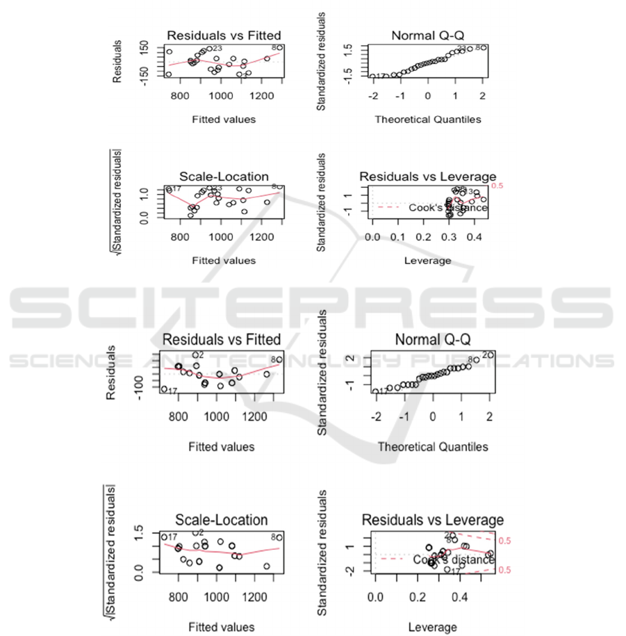
In order to check the three other regression
assumption, we decided to draw a set of diagnostic
plots According to the Normal QQ plot, we could see
only a few of the points fall long the dashed line. We
cannot conclude it’s almost normally distributed.
According to the Scale-Location plot, the residuals
spread without any specific patterns around
the red line,
but the red line is not as straight as expected, hence we
cannot assume for the constant variance. According to
the Residuals and Fitted plot, we found a decreasing
pattern for the distributed data, so the test for non-
linearity is not met. The residuals weren’t distributed
independently.
BDEDM 2022 - The International Conference on Big Data Economy and Digital Management
796
Since none of the regression assumptions are met,
there must be something wrong with the data. By
reviewing the data, the sample size is too small to
either construct unbiased analysis or maintain statistic
powers. Bootstrap, a technique for re-sampling might
help us to reduce these biases brought by small sample
sizes. Here we repeated 1000 times to construct a new
model.
Here, we draw four diagnostic plots again in Fig. 2
and found that even thought these plots are not
perfectly matched with regression assumption, they are
much better than the model we generated by only 24
data. Since the assumptions are almost met, the
Hypothesis test and Variable selection could be applied
in the following part.
Figure 1: The first 4-diagnostic plots.
Figure 2: The second 4-diagnostic plots.
The Impact of Marketing Mix’s Efficacy on the Sales Quantity based on Multivariate Regression
797

Table 4: Regression Results.
The
coefficients
intercept P
50
P
60
A
0
L
0
C
1
C
3
V
438.096 232.905 107.824 -268.098 -62.656 19.770 -5.270 12.204
Table 5: The First P-values for parameters.
P-Value
intercept P
50
P
60
A
0
L
0
C
1
C
3
V
0.073879 0.000254 0.033911 6.63e-05 0.092959 0.660419 0.932532 0.008625
Table 6: The Second P-values for parameters.
P-Value
intercept P
50
P
60
A
0
L
0
C
1
C
3
V P
50
:V P
60
:V
0.42790 0.29707 0.04658 0.00541 0.88797 0.35840 0.90640 0.01366 0.13293 0.07565
Table 7: Regression Results for new model.
The
coefficients
intercept P_50 P_60 A_0 C_1 V P_50:V P_60:V
207.891 -591.513 792.621 -175.677 -46.527 15.202 18.037 -14.042
3 RESULTS & DISCUSSION
The full Model is obtained based on regression, where
the coefficients values are listed in Table. IV. Here,
P
50
means that setting price at 50 could induce
232.905 more sales than setting price at 70, P
60
indicates that setting price at 60 could induce 107.824
more sales than setting price at 70, the A
0
denotes for
the 3 million advertising policy would bring 268.098
less sales than 3.5 million advertising policy, L
0
means that focusing on the Bakery section would
bring 62.656 less sales than that of Breakfast section,
C
1
is operating in city1 sell 19.770 more than
operating in city4, C
3
is operating in city3 sell 5.270
less than operating in city4 and V represents for each
unit increase in Store Volume is associated with an
increase of 12.204 in total sales.
To test whether these coefficients are statistically
significant, a Hypothesis test with significance level
is 0.1 will be used. H0: the coefficient is 0 and H1:
the coefficient is not 0
all the variable with corresponding p-value will be
compared with 0.1; if their p-value is less than 0.1, we
conclude that these variables are statistically
significant.
Based on the output summary, only C1 and C3
have extremely big P-value, which means these two
variables might be useless for the following analysis.
In order to figure out if the effect exsits, which
provided by different price, to the total sales depends
on the volumes, two interaction terms are added in
full model. The p-values results are given in Tables V
and VI.
The p-value for interaction between price at 60
and volumes is 0.07565, which is less than the
significance level (0.1), i.e., interaction term is
statistically significant. Even though one can tell
which variables affect the total sales by these full
model, it’s not good enough. In this case, a model
with less complexity is needed with more explained
variance. Less complexity means less terms in the
model, we want to make sure if there are any variables
we could remove. Here, we’ll refer to the notion of
Akaike information criterion, which compares the
quality for each model, with Stepwise Selection. The
model with the smallest AIC will be chosen.
BDEDM 2022 - The International Conference on Big Data Economy and Digital Management
798

The reduced model coefficients are given in
Table. VII. Another way to test the quality of two
models is to compare their coefficient of
determination (R squared), which measures the
proportion of total variation explained by the
regression model. With regard to deal with Multiple
Linear regression, the R squared is not accurate
enough since it would always increase when a new
variable is added to the model. We’ll focus on the
modified version (Adjusted R squared), which works
the as R squared. The larger the adjusted R squared
is, the better the model fit.
Table 8: Metics for the model.
Reduced Model (with
interaction)
Full Model (with
interaction)
AIC 206.41 210.34
R squared 0.8473 0.826
While viewing the variables of the model, we
could make another interpretation with interaction.
P
50
: If the company consider setting price at 50, they
will induce 519.513 less sales than setting price at 70.
P
60
: If the company consider setting price at 60, they
will induce 792.621 more sales than setting price at
70. A
0
: the 3 million advertising policy would bring
175.677 less sales than 3.5 million advertising policy.
C
1:
stores in city1 will bring 46.527 less sales than that
of city4. V: if the company considered setting price at
50, each unit increase in Store Volume is associated
with an increase of (15.202+18.037) in total sales. If
the company considered setting price at 60, each unit
increase in Store Volume is associated with an
increase of (15.202-14.042) in total sales. If the
company considered setting price at 70, each unit
increase in Store Volume is associated with an
increase of 15.202 in total sales.
According to the multiple linear regression, the
variables Price, Advertising, City Index, Store
Volume and interaction between Price and Store
Volume can determine the total sales of the Product–
K-pack. As a matter of fact, this regression model is
not perfect even though we did the bootstrap re-
sampling technique to reduce the bias. In the future,
if one could collect more data from the
SMARTFOOD company, a better regression analysis
can be formed, e.g., split data to carry out cross
validation and construct complex nonlinear model
(neural networks). The training data set would be
used to construct models and the test data set would
be used to evaluate the quality of linear models. Then,
the over-fitting problems might be eliminated and the
precision of regression analysis would be improved.
In addition, we need to reveal more variables which
might also affect the total sales of product. The more
variables the model includes, the better performance
one can obtain.
4 CONCLUSION
In summary, we investigate K-Pack’s 4-month
marketing performance based on multivariate linear
regression. According to the analysis, the feasibility to
sales prediction is verified and the impacts of efficacy
of marketing mix on the sales are demonstrated. In the
future, to construct a more robust and improve the
performance, we can consider more variables as well
as enlarging the sample quantities. Besides, it is
necessary to pay attention to the marketing strategy of
competitors, detect market changes timely as well as
given questionnaires to customers regularly Market is
full of change. we have to pay attention to everything
about it, i.e., the prediction will be more reliable and
closer to the fact. Overall, these results offer a
guideline for sales prediction for a specific case.
REFERENCES
Bakker, J., and M. Pechenizkiy. "2009 IEEE International
Conference on Data Mining Workshops Towards
Context Aware Food Sales Prediction." (2014).
Blech, et al. "Predicting Diabetic Nephropathy Using a
Multifactorial Genetic Model. " Plos One (2011).
Braga, J. P. , et al. "Prediction of the electrical response of
solution-processed thin-film transistors using
multifactorial analysis." Journal of Materials Science:
Materials in Electronics 30.11(2019).
Meeran, S. , K. Dyussekeneva , and P. Goodwin . "Sales
Forecasting Using Combination of Diffusion Model
and Forecast Market an Adaption of
Prediction/preference Markets." IFAC Proceedings
Volumes 46.9(2013): 87-92.
Meeran, S., K. Dyussekeneva, and P. Goodwin. sales
forecasting using combination of diffusion model and
forecast market -an adaption of prediction/preference
markets. 2013.
The Impact of Marketing Mix’s Efficacy on the Sales Quantity based on Multivariate Regression
799

Reinsel, G. . "Estimation and Prediction in a Multivariate
Random Effects Generalized Linear Model." Journal of
the American Statal Association 79.386(1984):406-
414.
Sarukhanyan, A. , et al. "Multifactorial Linear Regression
Method For Prediction Of Mountain Rivers Flow."
(2014).
Tsoumakas, G. . "A survey of machine learning techniques
for food sales prediction." Artificial Intelligence
Review 52.1(2019):441-447.
Xin, L., and R. Ichise. "Food Sales Prediction with
Meteorological Data — A Case Study of a Japanese
Chain Supermarket." Springer, Cham (2017).
Ye, J., Y. Dang, and Y. Yang . "Forecasting the
multifactorial interval grey number sequences using
grey relational model and GM (1, N) model based on
effective information transformation." Soft Computing
24.7(2020):5255-5269.
Zliobaite, I., J. Bakker, and M. Pechenizkiy . "Beating the
baseline prediction in food sales: How intelligent an
intelligent predictor is?." Expert systems with
applications 39.1(2012):p.806-815.
Zliobaite, I., J. Bakker , and M. Pechenizkiy. "Towards
Context Aware Food Sales Prediction." IEEE
International Conference on Data Mining Workshops
IEEE, 2009.
BDEDM 2022 - The International Conference on Big Data Economy and Digital Management
800
