
Predicting Visible Terms from Image Captions using Concreteness and
Distributional Semantics
Jean Charbonnier
a
and Christian Wartena
b
Hochschule Hannover, Germany
Keywords:
Information Retrieval, Concreteness, Distributional Semantics.
Abstract:
Image captions in scientific papers usually are complementary to the images. Consequently, the captions contain
many terms that do not refer to concepts visible in the image. We conjecture that it is possible to distinguish
between these two types of terms in an image caption by analysing the text only. To examine this, we evaluated
different features. The dataset we used to compute tf.idf values, word embeddings and concreteness values
contains over 700 000 scientific papers with over 4,6 million images. The evaluation was done with a manually
annotated subset of 329 images. Additionally, we trained a support vector machine to predict whether a term
is a likely visible or not. We show that concreteness of terms is a very important feature to identify terms in
captions and context that refer to concepts visible in images.
1 INTRODUCTION
In the NOA prject, we collected over 4.6 million im-
ages from scientific open access publications. The
nature of this image collection is completely different
from classical image collections, as a large proportion
of the images are close ups, X-Rays and CRT-scans,
etc. Thus image recognition is not a solution to anno-
tate these images and make them available for retrieval.
Instead we select words from the image captions and
from sentences referring to the image. We need to
include sentences mentioning the image since in many
publications the captions are extremely short and do
not contain any terms referring to visible concepts.
Annotation of the images with good keywords is in
turn important to organise the images and to enable
efficient search.
Image-caption pairs in scientific publications differ
in two ways from image-caption pairs in most datasets.
In the first place the nature of the images is differ-
ent from the kind of images in most image analysis
datasets (see e.g. Figure 1). In the second place, in
most datasets we have captions that describe the image.
In terms of Unsworth’s taxonomy (Unsworth, 2007),
the image and the caption are concurrent. For most
image-caption pairs extracted from scientific publica-
tions the image and the caption are (at least partially)
a
https://orcid.org/0000-0001-6489-7687
b
https://orcid.org/0000-0001-5483-1529
complementary and usually the text extends the image.
E.g. in Figure 2 we see that the caption gives a lot of
additional information that is not present in the image.
In a text that is complementary to the correspond-
ing image we will find terms that refer to concepts
visible in the image and terms that do not refer to
depicted concepts but deal with the additional, com-
plementary information. In the rest of the paper we
will call the former ones visible terms.
We believe that the text in a complementary image-
text pair gives some clear cues, what words are visible
terms and which are not. Besides typical patterns to
refer to concepts in the image, we expect to see word
concreteness (Paivio et al., 1968) as a key feature to
identifying these words. Thus, our main hypothesis is,
that for image-caption pairs in which text and image
are complementary, concepts in the text represented
by words with high concreteness values are likely to
appear in the image as well.
To verify this hypothesis, we used our corpus of
over 710 000 scientific papers to train word embed-
dings and generate values for concreteness and idf.
These where then tested on a manually annotated col-
lection of 239 images trying to predict, what terms
from the caption and from the surrounding text de-
scribe objects visible on the image. We do not analyse
the image in any way, but just want to understand the
text and get cues to find out which terms describe the
image and which terms give additional information. It
turns out that concreteness of a term is an important
Charbonnier, J. and Wartena, C.
Predicting Visible Terms from Image Captions using Concreteness and Distributional Semantics.
DOI: 10.5220/0011351400003335
In Proceedings of the 14th International Joint Conference on Knowledge Discovery, Knowledge Engineering and Knowledge Management (IC3K 2022) - Volume 1: KDIR, pages 161-169
ISBN: 978-989-758-614-9; ISSN: 2184-3228
Copyright
c
2022 by SCITEPRESS – Science and Technology Publications, Lda. All rights reserved
161
Image
Caption
Photographs displaying microwave irradiated
synthesis of titled compounds.
Terms
photograph, microwave, derivative, reaction
time, result, water, heat, substance, wall, sol-
vent, energy, molecule, mixture, rise, tempera-
ture, thermal conductivity, superheating, rotation,
radiation, research, biginelli reaction, thiourea,
attempt, powers, final product, targets, chloro-
form, ethyl acetate, factor, ranges, spectrum, ab-
sorption band, region, stretching, vibration, pro-
ton, signal
Figure 1: Image and caption from Sahoo, Biswa Mohan et al.
"Ecofriendly and Facile One-Pot Multicomponent Synthesis
of Thiopyrimidines under Microwave Irradiation", Journal
of Nanoparticles (doi:10.1155/2013/780786). With terms
extracted from caption and sentences referring to the image.
The bold terms were identified by the annotators as terms
representing concepts visible in the image.
predictor for a term to appear in the image. Moreover,
we see that inverse document frequency is not a good
predictor.
After discussing the related work in section 2 we
present our dataset in section 3. In section 4 we de-
scribe our approach how to select visual concepts fol-
lowed by a description of our results and finish in
section 6 with our conclusion and future work.
2 RELATED WORK
Unsworth (2007) studies the relations that can exists
between text and images and defines a classification of
image-text relations. These classes are investigated in
detail in (Martinec and Salway, 2005) and (Otto et al.,
2019).
Concept detection in images and automatic cap-
Image
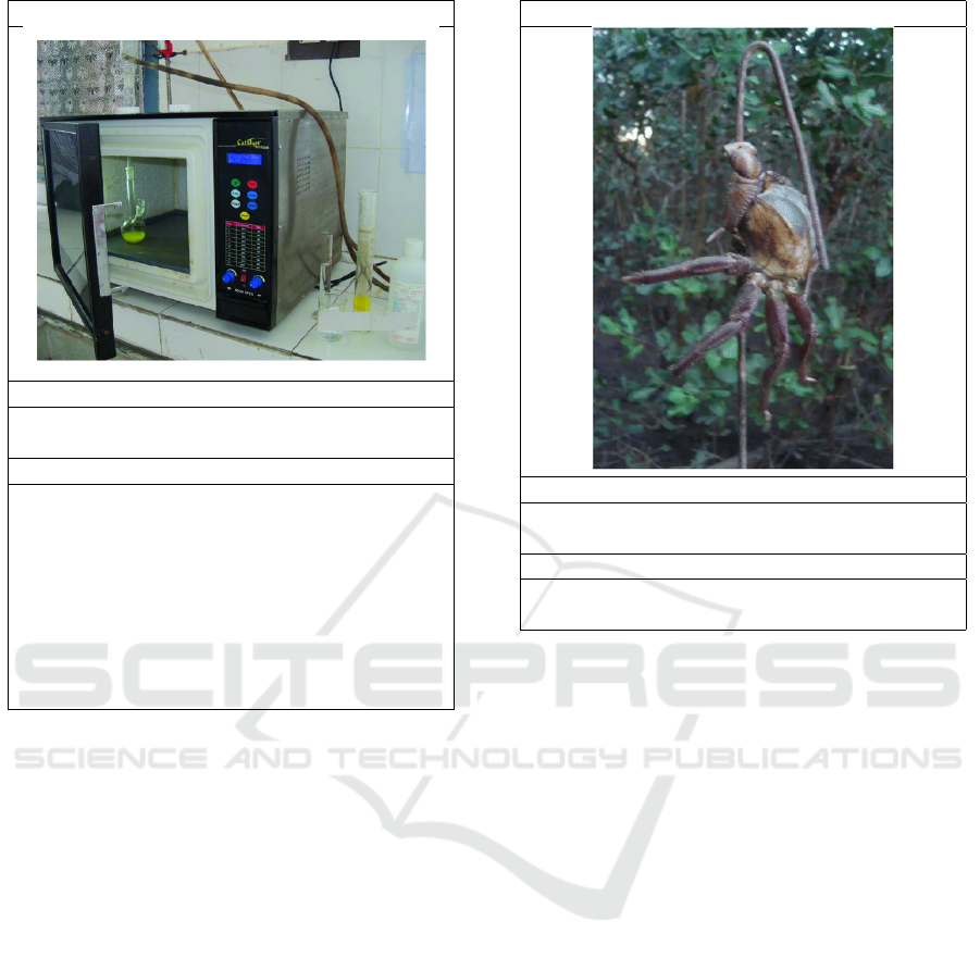
Caption
Fig. 2 Metal pole (hook) used to pull the crab out
by the catchers in Mucuri-Bahia State
Terms
figs, metal, poles, hook, crab, catcher, length,
burrow, productivity
Figure 2: Image and caption from Firmo, Angélica M.S.
et al. "Habits and customs of crab catchers in southern
Bahia, Brazil", Journal of Ethnobiology and Ethnomedicine
(doi:10.1186/s13002-017-0174-7). With terms extracted
from caption and sentences referring to the image. The
bold terms were identified by the annotators as terms repre-
senting concepts visible in the image.
tion generation is a very popular field of research. A
widely used dataset with image-caption pairs is Mi-
crosoft COCO (Lin et al., 2014). In this dataset all
captions were written as descriptions of the image.
Thus, these captions are not comparable to captions in
scientific papers. In fact, for COCO we can assume,
that each term mentioned in the caption refers to a
concept visible in the image: the relation between im-
age and text in COCO and similar datasets is a very
specific one, not suited to verify our hypothesis.
A huge amount of research was done on image
analysis and object and keyword detection using image
data. This is not the topic of the present paper. For
an overview of work in this area we refer to (Zhao
et al., 2019), who provides an overview of state of the
art methods of object detection with a focus on deep
learning.
Our goal to identify words referring to depicted
terms is most similar to keyword extraction. Algo-
rithms for keyword extractions are well researched.
Turney (2000) and Frank et al. (1999) used a decision
KDIR 2022 - 14th International Conference on Knowledge Discovery and Information Retrieval
162

tree to extract keyphrases based on various features in-
dicating the importance of a term. Besides the classic
features for salience and importance, inverted docu-
ment and term frequency Salton et al. (1975), they also
introduce new features like the position of a word in
the text and features indicating the ’keywordness’, the
suitability of a word as keyword.
Srihari et al. (2000) developed a multimedia in-
formation retrieval system, using various textual and
visual features from the images as well as from their
caption and context. For the image they used face
detection, colour histogram matching and background
similarity. From the text they extract named entities
and picture attributes using Wordnet and tf.idf weight-
ing. Gong et al. (2006) collected 12,000 web pages
with images which were annotated by 5 experts for
their topic. They select keywords for images by com-
bining the importance of a word in a text block and
the distance between the text block and the image.
Gong and Liu (2009) extend this idea and add features
from the images, especially textures generated by a
Daubechies wavelet transformation and a HSL color
histogram. These were then used to get positive and
negatives sets of images for words using a Gaussian
Mixture Model.
Leong and Mihalcea (2009) and Leong et al. (2010)
explore the possibility of automatic image annotation
using only textual features. They use features from
the text, like frequency (tf.idf) and the part of the text
in which the term occurs, as well as features of terms
computed on other datasets, like Flickr and Wikipedia.
These features should help to determine what words
are suited to describe images. Leong and Mihalcea
(2009) coin the likelihood of a term to be used as an
image tag on Flickr the Flickr picturability. Flickr
picturability seems to be very similar to concreteness
and visualness, two well studied properties of words
that are discussed below and that we will use to ex-
tract terms from captions. The main difference to our
work is the different nature of web images and images
from scientific papers. Flickr picturability does not
fit to our data, while concreteness is a more general,
domain independent concept and also not dependent
on a commercial black box API.
An important indicator for the likelihood of a con-
cept to appear in an image is the visualness of a con-
cept as pointed out by Jeong et al. (2012). Visualness,
often also called imageability or imagery, has been
studied extensively for decades in the psycholinguistic
community. Friendly et al. (1982) define visualness
as the ease to which a word arouses a mental image
when perceived. Visualness is one of the so called
affective norms that were determined experimentally
for many words. Many studies have shown a very
high correlation between visualness and concreteness
(Paivio et al., 1968; Algarabel et al., 1988; Clark and
Paivio, 2004; Charbonnier and Wartena, 2019). Since
much more data are available for concreteness, we will
use concreteness rather than visualness below. Brys-
baert et al. (2014) describe concreteness as the degree
to which a concept denoted by a word refers to a per-
ceptible entity; Similarly, Friendly et al. (1982) define
concrete words as words that "refer to tangible objects,
materials or persons which can be easily perceived
with senses". With the help of distributional similar-
ity between words or word embeddings as features
for words, it is possible to predict the concreteness
of words using supervised learning algorithms with a
very high accuracy (Turney, 2000; Charbonnier and
Wartena, 2019).
Concreteness has been used before in multimodal
datasets. Kehat and Pustejovsky (2017) use the occur-
rence of words in such a dataset to predict the con-
creteness of words. Similarly, Hessel et al. (2018)
determine a dataset specific concreteness for words
using image-text relations and show that retrieval per-
formance is higher for more concrete concepts.
3 DATASET
The dataset that we use for training contains full texts
from over 710k scientific papers and over 4.6 million
images and their captions from these papers. For eval-
uation 329 images from this collection were manually
annotated with concepts that are visible on the image
(visual terms) and general keywords that describe the
image but that are not necessarily depicted directly.
3.1 Source and Selection
In the NOA project 4.608 million images from 710 000
scientific publications were collected Most images
are charts, graphs, CT-scans, microscopy images etc.
About 10% of the collected images are photographs
(Sohmen et al., 2018). For each image we took the
image caption and all sentences with a reference to
that image. It was necessary to extend the captions
with referring sentences for two reasons. In the first
place in many publications the captions are too short,
consisting just of two or three words. In the second
place, even if the caption is meaningful, the context
might give additional synonyms and related terms that
can be helpful for further processing. From these ex-
tended captions we selected all terms that are used as a
title of an article in the English Wikipedia. Thus, terms
can be a single word or consist of multiple words. The
average number of terms extracted for the images in
Predicting Visible Terms from Image Captions using Concreteness and Distributional Semantics
163

the annotated data set is 25.22. The number of terms
per image ranges from 2 to 226. Table 1 gives the
numbers of terms extracted from the original captions
and from the context.
From the extracted terms the annotators selected
visible terms and keywords. In most cases the over-
lap between keywords and visible terms is very low:
the average Jaccard coefficient between keywords and
visible terms is 0.029.
3.2 Annotation
The images were annotated by two student assistants.
Only images that were classified as photographs were
presented to the annotators. The annotators were asked
to select visible terms from a list of candidate terms
and keywords, that do not necessarily denote depicted
concept, but are suited to characterise the image as a
whole.
The main guideline for selecting visible terms was
to select any term denoting a concept or thing that is
easily and clearly locatable on the image. I.e. there
should be a clear region on the image depicting the
term. E.g. if we have a picture of a bride and a groom
in a church, we can identify a bride, a priest, etc.,
but not a wedding. However, wedding would be a
good keyword. Usually objects, people, animals etc.
or parts of those turn out to be good candidates for
visible terms. On the other hand adjectives usually are
not suited as visible terms. Also general terms like
object, structure, sphere, surface, coloured are usually
not suited.
The second instruction was, that interpretation and
use of the common knowledge is allowed. If there is
e.g. a human with a shepherd’s crook, in front of sheep,
the term shepherd is justifiable.
For keywords the annotators were asked to select
terms that describe the image. Thus a term that is visi-
ble, but is not the main topic of the image should not
be selected. Here more general and abstract concepts
often fit very well.
The annotators were free to skip any image, but
each annotator was obliged to annotate all images se-
lected by the other annotator. We explicitly asked
the annotators to skip images consisting of several
sub-images and images containing text. Most other
skipped images were not annotated because the anno-
tators could not identify anything, either because of
bad image quality or because they were not familiar
with the technical objects on the picture. In total the
annotators selected descriptive terms for 329 images.
An example of an easy to annotate image with a small
number of terms is given in Figure 2.
The complete dataset of annotated images can be
downloaded from http://textmining.wp.hs-hannove
r.de/datasets. Table 2 gives an overview of the main
characteristics of the data set.
The annotation process was perceived as extremely
difficult and time consuming by the annotators, as they
were unfamiliar with many specific scientific terms.
Initially, both annotators selected visible terms and
keywords for each image. After this first annotation
phase the inter-annotator agreement measured by Krip-
pendorf’s
α
(Krippendorff, 1970) was
0.57
for key-
words and
0.58
for visual terms. Since the annotators
felt uncertain about their annotations for the visual
terms and were sure to have made many mistakes in
the first annotations, we have shown them all images
a second time. In this second phase they worked to-
gether, could discuss the annotations and remove in-
correctly selected terms but not add new terms to their
selection. The inter-annotator agreement for the visual
terms after this correction phase is
0.78
. In the follow-
ing we will always use the union of the selected terms
from both annotators, i.e. we consider a term as a good
visual term (respectively keyword) if it was selected
by one of the annotators.
4 SELECTING VISIBLE
CONCEPTS
One of the most common methods to select character-
istic terms from a text is to use the inverse document
frequency (idf). This is in fact a kind of unsupervised
learning, since the idf values of each term have to be
computed on a collection of training data, but without
any supervision. Other features can be computed in
a similar way. In the classical supervised keyword
extraction approach, discussed above, a supervised
method is used to combine these features in an opti-
mal way. This is of course only possible if enough
training data are available. In order to investigate the
potentials and usefulness of each feature, however, no
training data are required and a smaller set of test data
suffices. For keyword extraction from news texts or
abstracts of scientific papers idf is known to be always
one of the best features. In the following we will inves-
tigate whether this holds for image captions as well, or
whether other features give better results.
In order to evaluate features, we rank the terms
according to each feature and evaluate these rankings.
For some features we have many terms that get a de-
fault value for that feature. In these cases we cannot
sort the terms when we use only that feature. To solve
this problem, we always randomly shuffle all terms
with the same value.
KDIR 2022 - 14th International Conference on Knowledge Discovery and Information Retrieval
164

Table 1: Average number of terms from caption and context per image.
all data annotated data
terms terms vis. term keywords
caption only 6.15 3.31 0.29 0.45
context only 19.77 21.26 1.21 0.50
capt. + cont. 4.20 2.49 0.71 1.14
total 21.49 25.22 2.22 2.10
Table 2: Main characteristics of the data set of scientific
images, captions, extracted and selected terms.
Number of images 329
Number of extracted terms 8296
Number of selected visual terms 729
Number of selected keywords 691
Number of annotators 2
Inter-annotator agreement (vis. terms) 0.78
Inter-annotator agreement (keywords) 0.57
IDF. We compute the inverse document frequency
on the whole collection of 4.6 Million image terms,
where the set of image terms for each image consists of
all Wikipedia terms extracted from caption and refer-
ring text as described above. We compute the idf value
for a term
t
as
idf(t) = log
N−d f (t)
d f (t)
where
d f (t)
is the
number of documents containing
t
and
N
the total num-
ber of documents. As a feature we finally use the nor-
malized idf-value, that is computed as idf
n
(t) =
idf(t)
logN
.
Caption Similarity. In the sentences referring to the
image, but also in the caption, we might find words
that are not representative for the caption. We measure
the degree of representativity of a term
t
by computing
the cosine of the word embedding of
t
and the averaged
embedding of all words in the caption. For this pur-
pose we computed word embeddings using word2vec
(Mikolov et al., 2013) on the full text of over 2 million
papers in our collection.
Concreteness. We assume that concrete words in the
caption are more likely to refer to concepts depicted in
the image than abstract words (see also section 2). We
compute the concreteness of each term using a model
trained on the concreteness values for 37,058 words
from (Brysbaert et al., 2014) as described by Charbon-
nier and Wartena (2019). If, for some reason, we have
no word embeddings for a term, we cannot compute
the concreteness and use the average concreteness over
all words. For terms consisting of several words we
use the maximum of all concreteness values of the indi-
vidual words, assuming that a phrase becomes usually
more concrete when we add additional information.
Pattern. Many captions explicitly mention what is
depicted by using phrases like Picture of an X. In order
to exploit this information we search for the regular
expression:
(photograph(ie|y)?|ct|CT|view|scan|
picture|image)s? of (the|a|an)?
If both the pattern and a term
t
are found in the cap-
tion, we determine the position of the pattern,
pos
pat
,
and
pos(t)
the position of
t
in the caption. We use
1
pos(t)−pos
pat
as the value for this feature. If either the
term or the pattern is not found the value is
0
. For most
captions we do not find such a pattern and if the pat-
tern is found, most words usually come from referring
sentences and are not found in the caption. Thus this
feature usually is
0
. The pattern was found only in 18
of 329 captions and thus only can have a small impact
on the overall result.
Position. We assume that image captions follow a
structure where the beginning of the caption describes
the visible content of the image and the end gives more
explanation and back-ground information. Therefor
we expect to find the best visual terms/keywords in the
beginning of the caption and weight the terms relative
to their position using
1 −
pos(t)+1
len(caption)
. If the word is not
found in the caption the value is set to
−1
, which is the
case for a large fraction of all terms. The position of a
word in a text is also a common feature for keyword
extraction.
Source. As we can see in Table 1, terms that are
found as well in the caption as in the context are ex-
tremely likely to be a keyword or a visible term. Thus
we introduce a binary feature telling whether the term
was found in one (caption or context) or in two sources
(caption and context). Whether a term is found in the
caption or not is already coded indirectly in the fea-
tures Position and partially in Caption Similarity.
Predicting Visible Terms from Image Captions using Concreteness and Distributional Semantics
165

5 RESULTS AND DISCUSSION
5.1 Results
The effectiveness of each feature for extracting visible
terms and key terms in the test set is given in Table 3
and 4, respectively. Here we report the Area under the
ROC Curve (AUC) and precision and recall for the top
3 results. Furthermore, we also calculated Spearman’s
ρ
rank correlation between the results given by each
feature. These results are given in Table 5.
Table 3: Results for the prediction of visible terms. All
values are averages with their standard deviations from the
extraction for 329 captions.
Method AUC Prec@3 Rec@3
IDF 0.57 ± 0.23 0.16 ± 0.21 0.26 ± 0.38
similarity 0.67 ± 0.27 0.26 ± 0.26 0.39 ± 0.49
concr. 0.80 ± 0.19 0.25 ± 0.25 0.52 ± 0.38
pattern 0.52 ± 0.24 0.16 ± 0.21 0.25 ± 0.36
position 0.58 ± 0.25 0.22 ± 0.22 0.35 ± 0.38
source 0.64 ± 0.26 0.22 ± 0.22 0.37 ± 0.39
Table 4: Results for the prediction of keywords. All values
are averages with their standard deviations from the extrac-
tion for 317 captions.
Method AUC Prec@3 Rec@3
IDF 0.64 ± 0.23 0.22 ± 0.24 0.34 ± 0.37
similarity 0.74 ± 0.24 0.35 ± 0.27 0.49 ± 0.37
concr. 0.59 ± 0.25 0.20 ± 0.24 0.29 ± 0.35
pattern 0.54 ± 0.24 0.17 ± 0.23 0.26 ± 0.35
position 0.63 ± 0.26 0.29 ± 0.25 0.42 ± 0.36
source 0.72 ± 0.25 0.36 ± 0.89 0.51 ± 0.39
5.2 Discussion
For the kind of image-text pairs that we consider, we
find terms in the text (caption and sentences with an
explicit reference to the image) referring to concepts
visible in the image as well as to concepts not present
in the image. Our hypothesis was, that we can distin-
guish these terms by analysing only the text. We did
Table 5: Spearman correlation between results of each fea-
ture. For the binary features (pattern and source) results with
the same value are ordered randomly.
IDF sim. concr. pattern position
IDF -
sim. 0.328 -
concr. 0.194 0.142 -
pattern 0.017 0.010 0.004 -
position 0.021 0.067 0.065 0.029 -
source 0.057 0.184 0.058 0.057 0.174
not find a single feature that perfectly separates the
terms, but concreteness turns out to be a good predictor
for the appearance in the image: In Table 4 we see that
the ranking of terms only according to concreteness
already gives an AUC of 0.80. For selecting good key-
words concreteness is on contrary almost useless. If a
term is mentioned both in the caption and in referring
sentences, it seems indeed to be an important term for
the image and is highly likely to be either a key term
or a visible term. This feature is somewhat specific
for images in scientific papers, where we always have
a caption and explicit references to a figure. A fur-
ther good and more general feature for both extraction
tasks is the similarity of a word with the averaged word
vector of the terms in the caption.
The regular expression described in section 4 is
of course a strong indication if the pattern is present,
unfortunately in most captions no matching pattern is
found at all and thus this feature does not contribute
a lot to the result. Nevertheless, in an application it is
important to use this feature, as no user will understand
that a term X is not present as descriptive term while
the captions explicitly says that it is “a picture of X”.
The position of the word in the caption also seems to
be informative, as was noticed in various studies on
keyword extraction.
Interestingly, we see that inverse document fre-
quency is not a useful feature for the extraction of
visible terms. This contrasts almost all other appli-
cations of keyword extraction. The reason is clear,
when we look at the images and captions in more de-
tail: something quite general can be seen on the image,
e.g., an oak forest, but the caption uses a lot of specific
terms about experiments or observations not visible on
the picture. In a concrete example of such an image
(Figure 4 of https://www.hindawi.com/journals/isrn/20
11/787181/) the caption contains the following phrase
. . . sites selected for sampling in the wildlife bovine TB
transmission areas: (a) an oak forest where deer fecal
pellets were collected; . . . .
Finally, we see that almost all features are com-
pletely unrelated. For the binary features this is not
surprising since all results with the same feature value
were ordered randomly. Remarkable is the weak cor-
relation between the binary source feature and the sim-
ilarity of word embeddings from the keyword and the
caption: both methods favor frequent words and words
appearing in the caption over words only appearing in
the context. The highest correlation is found between
idf and the similarity feature. This suggests that the
influence of salient words on the average word em-
bedding of the caption is larger than that of common
words.
KDIR 2022 - 14th International Conference on Knowledge Discovery and Information Retrieval
166

5.3 Supervised Classification
Finally, we want to know how good a supervised classi-
fier would perform combining all features. The amount
of training data seems to be quite small. However, the
number of features is small as well and as we consider
the problem of selecting visible terms (and keywords)
as a binary classification problem (each term has to be
classified as being a visible term (or keyword) or not),
we have enough instances to train and evaluate a classi-
fier. As we have selected 8,296 candidate terms for all
images (see Table 2, we have in principle 8,296 cases
to train and evaluate the classifier on. Additionally,
the features for idf, word embeddings and concrete-
ness contain information from much larger datasets.
We evaluate the classifiers per image-caption pair and
compute typical measures like precision and recall per
image, since the overall accuracy of course is very
high due to the fact that almost every term is not a
visible term (or keyword).
As a simple, but robust and usually good classifier
we used logistic regression. We also trained Support
Vector Machines (SVM). We used a rbf kernel with the
following hyper parameters
1
, both for classification of
visual terms and key terms:
γ = 1 · 10
−2
,
C = 10
. In
order to rank the the binary classification results, we
sort the terms according to the confidence scores given
by the classifier.
The results for classification are given in Table 6.
If we compare these results to those in Table 3
and 4 we see that the combination of he features in-
deed gives better results. For the visible terms there
is only a moderate improvement of the AUC over the
result from concreteness only, emphasising again the
strength of this feature.
If we take a closer look at the results, in many cases
we find that the classifier selects a lot of terms that are
too general. E.g. we have an image of a milling cutter
and a setup for automatic visual analysis of a surface
(https://www.hindawi.com/journals/JOPTI/2015/
192030.fig.001b.jpg). Here only the term machine
was selected manually. While machine is already very
general, the classifier selects even more general terms:
’machine’, ’wear’, ’system’, ’tool’.
Another frequent type of error is, that the classifier
predict too many terms, as becomes clear when we
compare Table 1 with Table 6. A typical example is an
image showing the erosion of vegetation on the shore
after a tsunami (https://www.the-cryosphere.net/10/
995/2016/tc-10-995-2016-f07.jpg). The annotators
selected one visible term: cliff. The SVM predicted
a large number of very concrete terms, that indeed
are likely to appear on an image: ’glacier terminus’,
1
Determined using grid search
’shore’, ’port’, ’tsunami’, ’waves’, ’sea level’, ’beach’,
’lagoon’, ’vegetation’, ’boat’, ’birch’, ’bay’, ’cliff’,
’glacier’, ’shores’, ’ice’. Only shores is here a correct
suggestion, that, however, was not selected by the
annotators in this case.
We also trained a logistic regression classifier that
gave almost the same results as the support vector clas-
sifier. In addition now the coefficients learned for each
feature (see Table 7) give some additional insight in the
usefulness of each feature. The coefficients (though
computed only on a small part of the whole dataset)
confirm the picture that we already had: For finding vi-
sual terms concreteness turns out to be very important.
For the key terms the distributional similarity between
a keyword and the average of all caption words is the
feature with the highest weight. IDF is not important
for either of the tasks. Finally, the pattern looking for
an explicit phrase ’Picture of . . . ’ gets a high weight.
This is not contradicting the low performance of this
feature. If the feature is present, it is a very strong in-
dicator that the following word is depicted, but usually
the pattern is not found it gives no information.
6 CONCLUSIONS AND FUTURE
WORK
We have created a dataset with image-caption pairs
extracted from scientific open access publications. All
texts and images have a CC-BY or similar liberal copy-
right and can be reused freely. For each image we
extract concepts from the caption and from sentences
referring to the image. For each extracted concept two
annotators decided whether the concept is visible in
the image. The dataset differs from other datasets with
images and captions both in the nature of the images
and in the type of relation between image and text.
We have shown, that we can predict with a consid-
erable level of accuracy what terms from the text are
likely to represent concepts visible in the image with-
out analysing the image. We found that concreteness
of words is a key property for this prediction.
The extraction of visual terms and key terms was
used to annotate our dataset. Some of the images
from the dataset along with the extracted keywords
and categories derived from that were uploaded semi-
automatically to Wikimedia Commons (https://comm
ons.wikimedia.org/wiki/Category:Uploads
_
from
_
N
OA
_
project). Since all terms are titles from Wikipedia
articles we can collect the wikipedia categories of these
classes. Classes that are covering several keywords
and visual terms are very likely to fit well to the image
and are proposed as a category when the image was
uploaded.
Predicting Visible Terms from Image Captions using Concreteness and Distributional Semantics
167

Table 6: Results for the prediction of visible terms. All values are averages with their standard deviations from the extraction
for 329 captions (317 for keywords) using 5-fold cross validation.
Method AUC Prec Rec # of pred.
Vis. terms 0.84 ± 0.17 0.37 ± 0.28 0.80 ± 0.32 7.4 ± 8.6
Key terms 0.80 ± 0.24 0.44 ± 0.32 0.64 ± 0.38 4.4 ± 3.2
Table 7: Coefficients for features in the logistic regression
models.
Vis. Term Keyword
Feature Coefficient Coefficient
idf 0.00 ± 0.00 0.05 ± 0.01
caption similarity 3.75 ± 0.17 4.49 ± 0.18
concreteness 8.63 ± 0.18 0.47 ± 0.07
pattern 3.03 ± 0.67 1.57 ± 0.57
position 0.39 ± 0.03 1.03 ± 0.31
For future work we plan to use contextualised word
embeddings as features for the term classification. We
expect e.g. that the term Fish bone will have different
embeddings in the context Picture of a fish bone than
in the context . . . extracted from fish bone. We expect
that a classifier can use these differences to distinguish
depicted from other concepts.
REFERENCES
Algarabel, S., Ruiz, J. C., and Sanmartin, J. (1988). The
University of Valencia’s computerized word pool. Be-
havior Research Methods, Instruments, & Computers,
20(4):398–403.
Brysbaert, M., Warriner, A. B., and Kuperman, V. (2014).
Concreteness ratings for 40 thousand generally known
English word lemmas. Behavior Research Methods,
46(3):904–911.
Charbonnier, J. and Wartena, C. (2019). Predicting word
concreteness and imagery. In Proceedings of the 13th
International Conference on Computational Semantics
- Long Papers, pages 176–187, Gothenburg, Sweden.
Association for Computational Linguistics.
Clark, J. M. and Paivio, A. (2004). Extensions of the Paivio,
Yuille, and Madigan (1968) norms. Behavior Research
Methods, Instruments, & Computers, 36(3):371–383.
Frank, E., Paynter, G. W., Witten, I. H., Gutwin, C.,
and Nevill-Manning, C. G. (1999). Domain-Specific
Keyphrase Extraction. In Proceedings of the Sixteenth
International Joint Conference on Artificial Intelli-
gence, IJCAI ’99, pages 668–673, San Francisco, CA,
USA. Morgan Kaufmann Publishers Inc.
Friendly, M., Franklin, P. E., Hoffman, D., and Rubin, D. C.
(1982). The Toronto Word Pool: Norms for imagery,
concreteness, orthographic variables, and grammatical
usage for 1,080 words. Behavior Research Methods &
Instrumentation, 14(4):375–399.
Gong, Z., Cheang, C. W., et al. (2006). Web image indexing
by using associated texts. Knowledge and information
systems, 10(2):243–264.
Gong, Z. and Liu, Q. (2009). Improving keyword based
web image search with visual feature distribution and
term expansion. Knowledge and Information Systems,
21(1):113–132.
Hessel, J., Mimno, D., and Lee, L. (2018). Quantifying the
visual concreteness of words and topics in multimodal
datasets. In Proceedings of the 2018 Conference of
the North American Chapter of the Association for
Computational Linguistics: Human Language Tech-
nologies, Volume 1 (Long Papers), pages 2194–2205,
New Orleans, Louisiana. Association for Computa-
tional Linguistics.
Jeong, J.-W., Wang, X.-J., and Lee, D.-H. (2012). Towards
measuring the visualness of a concept. In Proceedings
of the 21st ACM international conference on Informa-
tion and knowledge management, pages 2415–2418.
ACM.
Kehat, G. and Pustejovsky, J. (2017). Integrating vision
and language datasets to measure word concreteness.
In Proceedings of the Eighth International Joint Con-
ference on Natural Language Processing (Volume 2:
Short Papers), pages 103–108, Taipei, Taiwan. Asian
Federation of Natural Language Processing.
Krippendorff, K. (1970). Estimating the reliability, system-
atic error and random error of interval data. Educa-
tional and Psychological Measurement, 30(1):61–70.
Leong, C. W. and Mihalcea, R. (2009). Explorations in
automatic image annotation using textual features. In
Proceedings of the Third Linguistic Annotation Work-
shop (LAW III), pages 56–59.
Leong, C. W., Mihalcea, R., and Hassan, S. (2010). Text
mining for automatic image tagging. In Coling 2010:
Posters, pages 647–655.
Lin, T.-Y., Maire, M., Belongie, S., Hays, J., Perona, P.,
Ramanan, D., Dollár, P., and Zitnick, C. L. (2014).
Microsoft coco: Common objects in context. In Euro-
pean conference on computer vision, pages 740–755.
Springer.
Martinec, R. and Salway, A. (2005). A system for image–text
relations in new (and old) media. Visual communica-
tion, 4(3):337–371.
Mikolov, T., Sutskever, I., Chen, K., Corrado, G., and Dean,
J. (2013). Distributed representations of words and
phrases and their compositionality. In Proceedings of
the 26th International Conference on Neural Informa-
tion Processing Systems - Volume 2, NIPS’13, pages
3111–3119, USA. Curran Associates Inc.
Otto, C., Springstein, M., Anand, A., and Ewerth, R. (2019).
Understanding, categorizing and predicting seman-
tic image-text relations. In Proceedings of the 2019
on International Conference on Multimedia Retrieval,
ICMR ’19, pages 168–176, New York, NY, USA.
ACM.
KDIR 2022 - 14th International Conference on Knowledge Discovery and Information Retrieval
168

Paivio, A., Yuille, J. C., and Madigan, S. A. (1968). Con-
creteness, imagery, and meaningfulness values for 925
nouns. Journal of Experimental Psychology, 76(1,
Pt.2):1–25.
Salton, G., Yang, C.-S., and Yu, C. T. (1975). A theory
of term importance in automatic text analysis. Jour-
nal of the American society for Information Science,
26(1):33–44.
Sohmen, L., Charbonnier, J., Blümel, I., Wartena, C., and
Heller, L. (2018). Figures in scientific open access
publications. In Méndez, E., Crestani, F., Ribeiro, C.,
David, G., and Lopes, J. C., editors, Digital Libraries
for Open Knowledge, pages 220–226, Cham. Springer
International Publishing.
Srihari, R. K., Zhang, Z., and Rao, A. (2000). Intelligent
indexing and semantic retrieval of multimodal docu-
ments. Information Retrieval, 2(2):245–275.
Turney, P. D. (2000). Learning Algorithms for Keyphrase
Extraction. Inf. Retr., 2(4):303–336.
Unsworth, L. (2007). Image/text relations and intersemio-
sis: Towards multimodal text description for multilit-
eracies education. In Proceedings of the 33rd IFSC:
International Systemic Functional Congress. Pontifícia
Universidade Católica de São Paulo.
Zhao, Z.-Q., Zheng, P., Xu, S.-t., and Wu, X. (2019). Ob-
ject detection with deep learning: A review. IEEE
transactions on neural networks and learning systems.
Predicting Visible Terms from Image Captions using Concreteness and Distributional Semantics
169
