
New Benchmarks and Optimization Model for the Storage Location
Assignment Problem
Johan Oxenstierna
1,2 a
, Jacek Malec
1b
and Volker Krueger
1c
1
Dept. of Computer Science, Lund University, Lund, Sweden
2
Kairos Logic AB, Lund, Sweden
Keywords: Storage Location Assignment Problem, Order Batching Problem, Quadratic Assignment Problem,
Warehousing, Computational Efficiency.
Abstract: The Storage Location Assignment Problem (SLAP) is of primary significance to warehouse operations since
the cost of order-picking is strongly related to where and how far vehicles have to travel. Unfortunately, a
generalized model of the SLAP, including various warehouse layouts, order-picking methodologies and
constraints, poses a highly intractable problem. Proposed optimization methods for the SLAP tend to be
designed for specific scenarios and there exists no standard benchmark dataset format. We propose new SLAP
benchmark instances on a TSPLIB format and show how they can be efficiently optimized using an Order
Batching Problem (OBP) optimizer, Single Batch Iterated (SBI), with a Quadratic Assignment Problem
(QAP) surrogate model (QAP-SBI). In experiments we find that the QAP surrogate model demonstrates a
sufficiently strong predictive power while being 50-122 times faster than SBI. We conclude that a QAP
surrogate model can be successfully utilized to increase computational efficiency. Further work is needed to
tune hyperparameters in QAP-SBI and to incorporate capability to handle more SLAP scenarios.
1 INTRODUCTION
The Storage Location Assignment Problem (SLAP)
concerns the “allocation of products into a storage
space and optimization of the material handling (…)
or storage space utilization [costs]” (Charris et al.,
2018). Material handling involves all processes
relating to the movement of products in a warehouse.
The location assignment of products thus has an
impact on the quality of material handling (Mantel et
al., 2007). For example, if a vehicle needs to pick a
set of products, the travel cost clearly depends on
where the products are located. At the same time, the
opposite is true in that material handling has an
impact on location assignment: Vehicle constraints,
traffic rules and picking methodologies can all have
an impact on how a strong location assignment is
formulated in the first place.
Kübler et al. (2020) describe a “joint storage
location assignment, order batching and picker
routing problem” where the SLAP includes two
a
https://orcid.org/0000−0002−6608−9621
b
https://orcid.org/0000−0002−2121−1937
c
https://orcid.org/0000−0002−8836−8816
interlinked optimization problems in the warehouse:
In the Order Batching Problem (OBP) vehicles are
assigned to carry sets of orders (each order contains a
set of products) (Koster et al., 2007). In the Picker
Routing Problem the picking path of a vehicle is
decided and it is equivalent to a Traveling Salesman
Problem (TSP) (Ratliff & Rosenthal, 1983). This
paper builds on Kübler et al.’s joint formulation and
we treat the Key Performance Indicator (KPI) in both
OBP and SLAP optimization as an estimate of
aggregate travel in the warehouse. The key difference
between the OBP and SLAP in this regard is that all
products are assumed to have fixed locations in the
former, whereas a subset of products are assumed to
be available for location assignment or reassignment
in the latter.
The main focus of this paper is two areas where
the SLAP has not seen much previous work. The first
area is that of benchmarking. Currently there is a
scarcity of benchmark data on any version of the
SLAP, and existing datasets are on various formats,
26
Oxenstierna, J., Malec, J. and Krueger, V.
New Benchmarks and Optimization Model for the Storage Location Assignment Problem.
DOI: 10.5220/0011378400003329
In Proceedings of the 3rd International Conference on Innovative Intelligent Industrial Production and Logistics (IN4PL 2022), pages 26-35
ISBN: 978-989-758-612-5; ISSN: 2184-9285
Copyright
c
2022 by SCITEPRESS – Science and Technology Publications, Lda. All rights reserved

making them difficult to reproduce (Section 2). We
propose new benchmark instances using
modifications to the wide-spread TSPLIB format
(Reinelt, 1991) (Section 5). A key discussion
regarding benchmark instances is how they can be
kept as simple and standardized as possible, to enable
easy reproducibility, while not losing applicability
within the industry. One benchmarking area which is
particularly difficult to standardize is the “relocation
efforts” for different types of SLAP assignment
scenarios (Section 2). We have delimited our SLAP
model to assignment scenarios where products are
hitherto not located in the warehouse.
The second focus area is the maximization of
computational efficiency in OBP optimization. As
mentioned above, a feature in the proposed model is
that an OBP is used to estimate the quality of SLAP
location assignments. Since the OBP is NP-hard it
must be optimized in a way which trades off solution
quality with CPU-time. We use the computationally
efficient OBP optimizer Single Batch Iterated (SBI)
(Oxenstierna, Malec, et al., 2021; Oxenstierna et al.,
2022). Within the proposed SLAP optimizer, SBI still
requires a lot of CPU-time and we investigate
whether it can be assisted by a Quadratic Assignment
Problem (QAP) surrogate model to make
optimization more efficient. The contributions are as
follows:
1. Introduction of SLAP benchmark data on the
TSPLIB format.
2. Feasibility analysis of a QAP surrogate model
within a SLAP optimizer.
2 LITERATURE REVIEW
This section goes through general strategies for
conducting storage location assignment and ways in
which their quality can be evaluated. Various SLAP
formulations and proposed optimization algorithms
are covered. We mainly concern ourselves with a
standard picker-to-parts set up and we particularly
refer to Kubler et al. (2020), since their proposed
model shares similarities with ours.
There exist numerous general strategies for
conducting storage location assignment (Charris et
al., 2018). Three key strategies are Dedicated, Class-
based and Random storage:
• Dedicated: Each product is assigned to a specific
location which never changes. This strategy is
suitable if the product collection changes rarely and
simplicity is desired. Human pickers can furthermore
benefit from this strategy since they can learn to
associate specific products with locations, which
might speed up their picking (Zhang et al., 2019).
• Random: Each product can be assigned any
available location in the warehouse. This is suitable
whenever the product collection changes frequently.
• Class-based (zoning): The warehouse is divided
into zones and the products into classes (usually
based on demand of products). Each class is assigned
a zone. The outline of the zone can be regarded as
dedicated in that it does not change, whereas the
placement of each product in a zone is assumed to be
random (Mantel et al., 2007). Class-based storage
assignment can therefore be regarded as a middle
ground between dedicated and random.
The quality of a location assignment is commonly
evaluated based on some model of aggregate travel
cost. For this purpose, a simplified simulation of
order-picking in the warehouse can be used (Charris
et al., 2018; Mantel et al., 2007). Some proposals
include the simulation of order-picking by the so
called Cube per Order Index (COI) (Kallina & Lynn,
1976). COI includes the volume of a product and the
frequency with which it is picked (historically or
forecasted). The general idea is then to assign
products with high pick frequency and relatively low
volume to locations close to the depot. Since orders
may contain products which are not located close to
each other, COI is only capable of simulating an
order-picking scenario adequately where orders
contain one product and vehicles carry one product at
a time. This may be sufficient when trucks pick a
couple of pallets or when certain types of robots are
used (Azadeh et al., 2019). Mantel et al. (2007),
introduced Order Oriented Slotting (OOS) where
vehicles are assumed to pick one order at a time, but
where the number of products in an order may be
greater than 1. They also introduce a Quadratic
Assignment Problem (QAP) model to estimate the
quality of a product location assignment, which
includes the distance between the product locations in
the order and a single depot location. A similar model
to OOS is used by Fontana & Nepomuceno (2017),
Lee et al. (2020) and Žulj et al. (2018).
There is not much prior research on SLAP’s
where vehicles are assumed to pick more than one
order at a time, i.e., where OBP optimization in some
form is included in SLAP optimization. We are only
aware of two papers within this category. The first is
Kübler et al. (2020), whose work we discuss further
below. The second is Xiang et al. (2018), but their
work concerns a robotic warehouse where the
vehicles are pods (moving racks) and is not easily
comparable to a picker-to-parts system.
New Benchmarks and Optimization Model for the Storage Location Assignment Problem
27

Travel cost is not the only way in which a SLAP
solution quality can be evaluated. Lee et al. (2020),
for example, study the effect of location assignment
and traffic congestion in the warehouse. If too many
products are assigned locations close to the depot (the
goal in common COI), there may be a traffic
congestion problem and it should ideally be included
in an industrially adopted model. They call their
version Correlated and Traffic Balanced Storage
Assignment (C&TBSA) and they formulate it as a
multi-objective problem with travel cost on the one
hand, and traffic congestion avoidance on the other.
Larco et al. (2017) study the relationship between
worker welfare and storage location assignment. If
picking is conducted by humans who move products
from shelves onto a vehicle, the weight and volume,
as well as the height of the shelf the product is placed
on, can have an impact on worker welfare. Worker
welfare can be quantified with parameters such as
“ergonomic loading”, “expenditure of human energy”
or “worker discomfort” (Charris et al., 2018).
The SLAP can be divided into two broad
categories depending on the number of location
assignments sought. Either the assignment is a “re-
warehousing” operation, which means that a large
portion of the warehouse’s products are (re)assigned
locations (Kofler et al., 2014). Most often, and more
realistically, however, only a small number of
products are (re)assigned a location and this is called
“healing” (Kofler et al., 2014). Solution proposals
involving healing often look closely at different types
of scenarios for carrying out initial assignments or
reassignments. Below are four scenarios presented by
Kübler et al. (2020):
I. Empty storage location: A product is
assigned to a previously unoccupied
location.
II. Direct exchange: A product changes
location with another product.
III. Indirect exchange 1: A product is moved to
another location which is occupied by
another product. The latter product is moved
to a third, empty location.
IV. Indirect exchange 2: A product is moved to
another location which is occupied by
another product. The latter product is moved
to a third location which is occupied by a
third product. The third product is moved to
the original location of the first product.
The above relocation scenarios are all associated
with different efforts, ranging from the lightest in
scenario I, to the heaviest in scenario IV. Kübler et al.
quantify efforts by considering both physical and
administrative times, which are transformed to effort
terms by proposed proportionalities. Total effort is
computed based on distances between old and new
locations for products and the total physical and
administrative efforts.
Concerning SLAP optimizers, proposals include
exact models such as Mixed Integer Linear
Programming (MILP), dynamic programming and
branch and bound algorithms (Charris et al., 2018).
The warehouse environment modeled in these studies
are simplified to a large extent (Charris et al., 2018;
Garfinkel, 2005; Kofler et al., 2014; Larco et al.,
2017). The main simplification concerns the above-
mentioned modeling of order-picking using COI or
OOS. Other simplifications involve limiting the
number of products (Garfinkel, 2005), number of
locations (Wu et al., 2014), or by requiring the
conventional warehouse rack layout (Kübler et al.,
2020). The conventional layout assumes Manhattan
style blocks of aisles and cross-aisles and it is used
almost exclusively in existing SLAP literature (we are
only aware of two exception cases using the
“fishbone” and “cascade” layouts (Cardona et al.,
2012; Charris et al., 2018).
Most proposed SLAP optimizers provide non-
exact solutions using heuristics or meta-heuristics.
These include multi-phase optimization where the
first phase evaluates possible locations for products
and the second phase carries out and evaluates the
possible assignments (Wutthisirisart et al., 2015). In
the meta-heuristic domain there are proposals
involving Genetic and Evolutionary Algorithms (Ene
& Öztürk, 2011; Lee et al., 2020), Simulated
Annealing (Zhang et al., 2019) and Particle Swarm
Optimization (PSO) (Kübler et al., 2020). In Kübler
et al. (2020), a heuristic zoning optimizer is used to
generate location assignments and a Discrete
Evolutionary Particle Swarm Optimizer (DEPSO) is
used to optimize the OBP (used as order-picking
model). DEPSO is a modification of a standard PSO
algorithm where the evolutionary part mitigates risk
of convergence on local minima. The discrete part
breaks the requirement of a continuous search space,
which is a requirement in standard PSO. If TSP
optimization is desired within a SLAP, S-shape or
Largest Gap algorithms (Roodbergen & Koster,
2001) are often used. For unconventional layouts with
a pre-computed distance matrix
Google OR-tools or
Concorde have been proposed for TSP optimization
(Oxenstierna et al., 2022; Rensburg, 2019).
IN4PL 2022 - 3rd International Conference on Innovative Intelligent Industrial Production and Logistics
28

3 PROBLEM FORMULATION
3.1 SLAP Model
The objective function of the SLAP model is similar
to the ones formulated in Henn & Wäscher (2012) and
Oxenstierna, van Rensburg, et al. (2021): Minimize
the distance needed to pick a given set of orders, using
order-batching:
𝑚𝑖𝑛 𝐷
(
𝑏
)
𝑎
,
∈ℬ
𝑚∈
ℳ
,ℬ⊂2
𝒪
(1)
where 𝒪 denotes orders, where ℬ denotes generated
batches, where 𝐷
(
𝑏
)
denotes the distance to pick
batch 𝑏 (the distance of a TSP solution) and where 𝑚
denotes a vehicle. 𝑎
denotes a binary variable that
is 1 if vehicle 𝑚 is assigned to pick 𝑏 and 0
otherwise. Products 𝒫 belong to orders 𝒪∈2
𝒫
and
the locations of all products in any order 𝑜∈𝒪 are
retrievable with function 𝑙𝑜𝑐
:𝒪→2
ℒ
𝒫
. ℒ
𝒫
denotes
all product locations in the warehouse. Similarly, all
locations in a batch of orders are retrievable using
function 𝑙𝑜𝑐
:ℬ→2
ℒ
𝒫
. The formulation is built on a
digitization pipeline for warehouses on any 2D rack-
layout, mapping of products to location coordinates,
precomputation of all shortest distances between
locations using the Floyd-Warshall graph algorithm,
constraints for order-integrity and vehicle capacities,
depot configurations and number of vertex visits.
Comprehensive details for warehouse digitization
and preprocessing for the OBP are beyond the scope
of this paper, so for details we refer to Oxenstierna,
van Rensburg, et al., (2021) and Rensburg (2019). As
mentioned in Section 1, the main difference between
the OBP and SLAP formulations concerns the
definition of product locations. In Oxenstierna, van
Rensburg, et al. (2021) each product 𝑝 ∈ 𝒫 “has a
[fixed] location”. We change this for the SLAP such
that a subset of products 𝒫
⊂𝒫 have their locations
removed in the warehouse. The SLAP then consists
of minimizing the OBP objective in Equation (1)
while trying various location assignments for 𝒫
.
The above SLAP scenario is represented by the
“empty storage location” scenario I in Kübler et al.
(2020) (Section 2). The relocation effort needed to
place the products at their assigned locations can be
assumed insignificant in this scenario, since finding
empty locations for new products in a warehouse is
not optional, but a requirement. The other of Kübler
et al.’s scenarios are “reassignments”, which means
that that the potential gains in travel cost due to
location reassignment must be weighed against the
cost of reassigning them. Including reassignments
makes a SLAP optimization model more complete,
but arguably also more complex. One of the aims of
this paper is to propose a model which allows for a
relatively simple and standardized SLAP benchmark
instance format. Contrary to Kübler et al., we chose
not to include various assignment scenarios in our
model, but on the other, we do not require a specific
warehouse layout. We invite further discussions on
how to rank and choose SLAP modeling features for
a standardized format.
3.2 QAP Model
Since Equation 1 poses an NP-hard problem, it would
require an infeasible amount of CPU-time to re-run
the minimization for a large number of candidate
solutions (location assignments). We therefore
propose to filter out promising candidates based on a
surrogate model. For this purpose we use a Quadratic
Assignment Problem (QAP) model with the
following objective:
𝑚𝑖𝑛 𝑤
∈ℒ
𝒫
∈ℒ
𝒫
∈𝒫
𝑑
×
∈𝒫
×𝑎
(
𝑝
,𝑙
)
𝑎
(
𝑝
,𝑙
)
(2)
where 𝑤 denotes weight, where 𝑑 denotes distance
and 𝑎
(
𝑝,𝑙
)
a function which returns 1 if product 𝑝 is
located at location 𝑙 and 0 otherwise. Cost is the
element-wise summation of a weight matrix and a
distance matrix. The cell values in the weight matrix
represent the number of times two products, 𝑝
,𝑝
,
appear in the same order 𝑜∈𝒪. The distances
between all product locations is assumed pre-
computed according to (Rensburg, 2019). If the
matrix indices for products in 𝒫
are permuted in such
a way that the aggregate distance and weights
between them is decreased, the QAP cost should also
decrease.
The intention with the QAP surrogate is then to
apply it in an accept/reject Markov Chain Monte
Carlo (MCMC) method (Cai et al., 2008). A sample
(solution candidate) 𝑥 should only be accepted if its
QAP cost estimate 𝑓
(
𝑥
)
(Equation 2) is low and close
to a corresponding OBP ground truth value 𝑓
∗
(
𝑥
)
(Equation 1). Assuming 𝑓
(
𝑥
)
and 𝑓
∗
(
𝑥
)
are
proportional, the accept probability can be upper
bounded by the following quotient (Christen & Fox,
2005):
𝑔
𝑓
(
𝑥
)
,
𝑓
∗
(
𝑥
)
≤
1
1+ 𝑒
|
(
)
∗
(
)|
(3)
New Benchmarks and Optimization Model for the Storage Location Assignment Problem
29

where 𝑔𝑓
(
𝑥
)
,𝑓
∗
(
𝑥
)
denotes the accept probability
and 𝐶 and 𝑃 positive constants. Unfortunately,
Equation 3 cannot be directly utilized in our case.
Since sample 𝑥 in the SLAP is a permutation of
arbitrary length (henceforth 𝒙), it would require an
infeasible amount of CPU-time to establish
proportionality between 𝑓 and 𝑓
∗
so that norm
|
𝑓
(
𝑥
)
−𝑓
∗
(
𝑥
)|
generalizes. Below we describe two
proposals for how this problem can be resolved.
If we have a dataset of finite samples with
available ground truth costs Ψ=𝒙,
𝑓
∗
(
𝒙
)
∈𝑿
×
ℝ
,𝑛∈ℤ, and a task where a single sample (e.g. the
best) should be found, a basic model of
proportionality between 𝑓 and 𝑓
∗
is provided by
softmax cross-entropy (Bruch et al., 2019; Cao et al.,
2007):
ℙ
𝑓
(
𝒙
)
=
𝑒
(𝒙
)
∑
𝑒
𝒙
(4)
ℙ
𝑓
∗
(
𝒙
)
=
𝑓
∗
(𝒙
)
∑
𝑓
∗
𝒙
(5)
𝐿
(
𝑓
)
=−
1
|
Ψ
|
ℙ
𝑓
∗
(
𝒙
𝑖
)
𝑙𝑜𝑔ℙ
𝑓
(
𝒙
𝑖
)
𝒙
𝒊
,
∗
(
𝒙
𝒊
)
∈
(6)
where ℙ𝑓
(
𝒙
)
and ℙ𝑓
∗
(
𝒙
)
denote the estimated
and ground truth probabilities of producing a sample,
respectively. 𝐿
(
𝑓
)
is the loss of 𝑓 (i.e., its distance to
𝑓
∗
). This model can be extended into Normalized
Discounted Cumulative Gain (NDCG) (Bruch et al.,
2019):
𝑁𝐷𝐶𝐺 =
𝐷𝐶𝐺
𝐼𝐷𝐶𝐺
(7)
𝐷𝐶𝐺 =
𝑓
(
𝒙
)
𝑙𝑜𝑔
𝜋
(
𝒙
)
(
𝑖
)
+1
(8)
𝐼𝐷𝐶𝐺 =
𝑓
∗
(
𝒙
)
𝑙𝑜𝑔
𝜋
𝑓
∗
(
𝒙
)
(
𝑖
)
+1
(9)
where 𝑓
(
𝒙
)
and 𝑓
∗
(
𝒙
)
denote relevance values
proportional to the approximated and ground truth
values in 𝑓
(
𝒙
)
and 𝑓
∗
(
𝒙
)
, respectively.𝜋 denotes a
ranking (a list of integers between 1 to 𝑛). 𝐼𝐷𝐶𝐺
denotes an ideal value where 𝑓
∗
(
𝒙
)
>𝑓
∗
(
𝒙
)
>
⋯>𝑓
∗
(
𝒙
)
. Bruch et al. (2019) argue that NDCG is
a stronger choice than softmax cross-entropy
whenever 𝑓
∗
is of non-binary type, which is the case
in Equation 1. We thus use NDCG to provide a
distance estimate between Equation 1 ( 𝑓
∗
) and
Equation 2
(
𝑓
)
. Choices for datatype for 𝑓
are
further discussed in the experiments in Section 5. In
Figure 4 (Appendix) an example is shown where
NDCG is computed from an input vector with range
1,𝑛
where 𝑛 denotes the number of solution
candidates (samples).
4 OPTIMIZATION ALGORITHM
The proposed optimization algorithm (QAP-SBI)
includes a module for SLAP candidate solution
generation and two estimators of solution quality: A
fast but noisy estimator using a Quadratic Assignment
Problem (QAP) model, and a slow but accurate Order
Batching Problem (OBP) optimizer (SBI):
Figure 1: Optimization model.
The input in step i is a future-predicted set of orders
𝒪 with products 𝒫 and 𝒫
⊂𝒫 (Section 3).
Predicting future orders is beyond the scope of this
paper and we assume this set already exists. See
Kübler et al. (2020) for an example of how prediction
of future orders can be carried out. In step ii 𝑛 SLAP
candidate solutions (for 𝒫
) are generated using basic
zoning (Section 2), stochasticity and a volume
capacity parameter. The pseudocode below describes
this procedure:
IN4PL 2022 - 3rd International Conference on Innovative Intelligent Industrial Production and Logistics
30
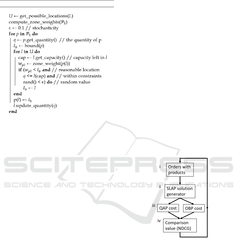
Algorithm 1: Assignment generation.
U is a set of locations which are not filled to capacity
in the warehouse and product 𝑝∈𝒫 must fit within
the location capacity constraint. A “zone weight” is
calculated to provide a probability that the product
should be assigned to a certain zone, depending on the
weight to other products in the same zone (using the
same weights matrix as described in Section 3). In the
rest of the procedure possible locations for the
products are iterated and a suitable SLAP candidate
is finally selected.
The solution costs of the candidate assignments
are estimated using the QAP model (step iii in Figure
1). In step iv the candidate solutions with the
strongest QAP estimates are selected and submitted
to OBP optimization in step v. We use the OBP
optimizer Single Batch Iterated (SBI) and its main
features are its high computational efficiency and its
ability to handle warehouses with unconventional
rack layouts (Oxenstierna et al., 2022). SBI only has
optimality bounds for small instances, so the quality
of its results for larger instances can be debated (as
far as we are aware there exists no proposal for how
to obtain optimal results for such instances within
feasible CPU-time). OBP optimization is beyond the
scope of this paper and we here treat SBI primarily as
a black-box which outputs ground-truth costs for
Equation 1. Steps ii, iii, iv and v are repeated until a
final timeout in step vi, when the candidate with
minimal OBP cost is selected as the best solution.
The algorithm in Figure 1 is an adaptation of the
MCMC sampling algorithm proposed by Christen &
Fox (2005), with two major differences: 1. CPU-time
parameters are used to dictate total number of
produced samples instead of convergence. 2. Step iv
selects multiple candidate solutions rather than one.
The latter step provides a convenient method with
which to validate the performance of the QAP model:
If all samples are accepted in iv and submitted to SBI
estimation, the predictive strength of the QAP model
can be easily evaluated.
In Figure 1 we note that steps iii and iv will be
useless for the overall optimizer if iv outputs random
candidate solutions. Steps iii and iv should therefore
perform better than a random baseline to be of use
(Freund et al., 2003; Freund & Schapire, 1996). In
Section 5 we follow this track and propose an
experimental set up where the QAP model is
benchmarked against a random baseline.
5 EXPERIMENTS
5.1 Experimental Set up
The main aim of the experiment is to empirically
validate the predictive strength of the QAP model
against ground truth values obtained through OBP
optimization. The diagram below shows the
experimental set up:
Figure 2: The modules in the experimental set up.
A test-instance is loaded in step i (orders with
products). In step ii, 𝑛 SLAP solution candidates are
generated semi-stochastically according to Algorithm
1. In step iii the cost of the generated solutions is
estimated using the QAP model and the OBP
optimizer SBI. The predictive strength of the QAP
model is defined as its ability to rank the solution
candidates according to NDCG (Section 3); 𝐼𝐷𝐶𝐺 is
computed from the ranking of costs according to the
OBP optimizer and 𝐷𝐶𝐺 is computed from the
ranking of costs according to the QAP model.
Relevance values 𝑓
(
𝒙
)
and 𝑓
∗
(
𝒙
)
are chosen to be
New Benchmarks and Optimization Model for the Storage Location Assignment Problem
31
the ranking of samples 𝒙 according to respective cost
functions. For 𝑛 candidate solutions the values are
defined as 𝑓
∗
(
𝒙
)
=(𝜋
∗
(
𝒙
)
(
𝑛
)
,𝜋
∗
(
𝒙
)
(
𝑛−
1
)
,…,𝜋
∗
(
𝒙
)
(
1
)
) and 𝑓
(
𝒙
)
=(𝜋
(
𝒙
)
(
𝑛
)
,𝜋
(
𝒙
)
(
𝑛−
1
)
,…,𝜋
(
𝒙
)
(
1
)
) (this corresponds to the set up shown
in Figure 4).
5.2 Benchmark Datasets
The TSPLIB format datasets (Reinelt, 1991) in
L6_203
1
and L09_251
2
are modified for the SLAP
and publicly shared in L17_533
3
. L17_533 includes
instances with one conventional and 5
unconventional warehouse obstacle layouts, various
depot configurations and vehicle capacities. The
number of orders range from 4 to 1000 and number
of products range between 10 to 3000. The SLAP
modification of the instances includes the tagging of
a number of products for storage assignment (𝒫
in
Section 3 and “SKUsToSlot” in the instance set). The
tag “assignmentOptions” is also added and includes
tagging of locations for assignment and how cost is to
be computed (it is always set to the “empty storage
location” scenario, Section 2). For analysis, instances
are divided into classes according to vehicle
capacities, number of orders and products and
number of candidate solutions. The global best OBP
result is tracked and then uploaded as the current
benchmark result for the corresponding instance. We
refer to the documentation in L17_533 for further
details. All instances are optimized using Intel Core
i7-4710MQ 2.5 GZ 4 cores, 16 GB RAM.
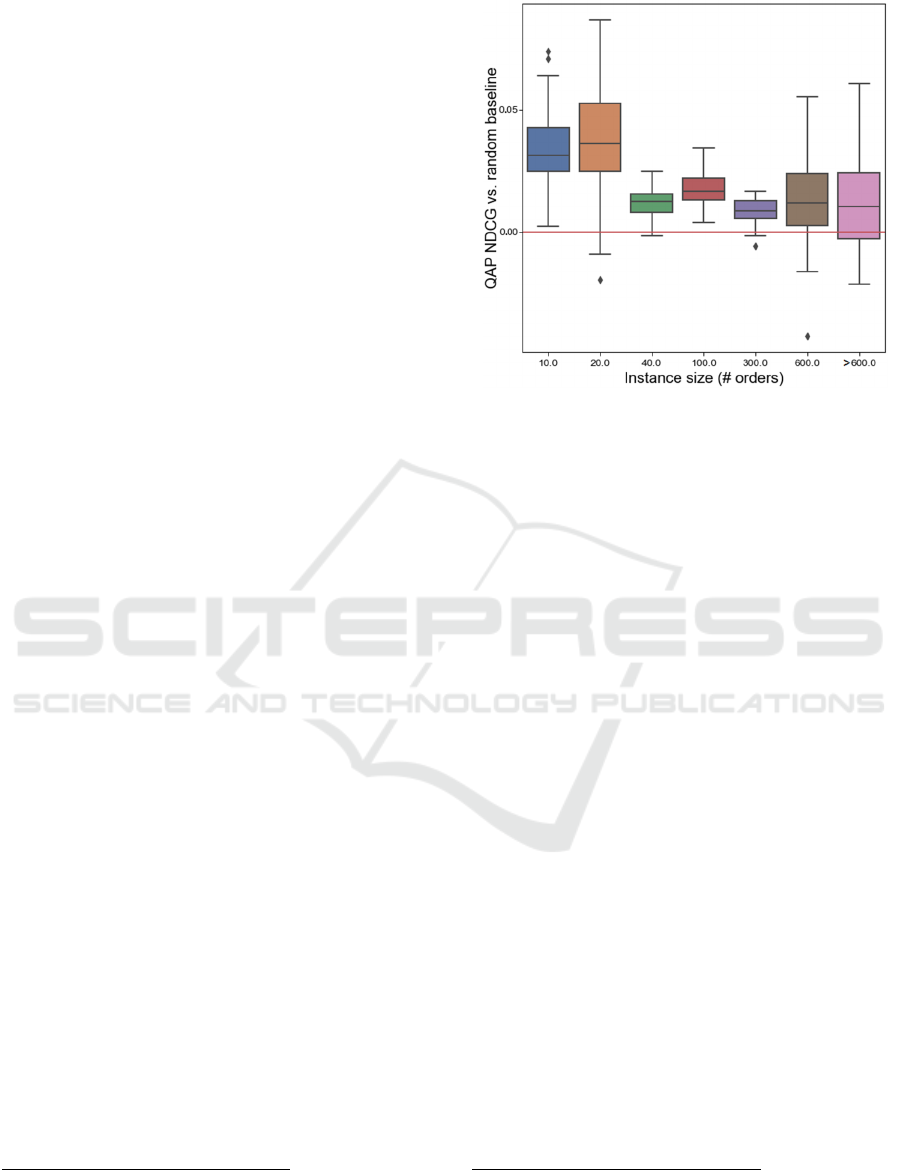
5.3 Experiment Result
Figure 3 and Table 1 summarize the results of the
QAP NDCG estimates versus the random value
baseline. On average, the QAP NDCG values are in
the range 0.83-0.90 (average over six 𝑛 values). They
are generally better than the random value baseline by
1-3%, with standard deviations ranging between 0.5-
2% (Figure 3). Most QAP estimates beat the random
baseline, but there are numerous exceptions,
especially for larger instances. The fraction of CPU-
time required by the QAP model versus the OBP
optimizer is between 0.008-0.019, meaning that it is
50-122 times faster. Table 1 also shows that this ratio
grows with instance size.
1
https://github.com/johanoxenstierna/OBP_instances,
collected 23-01-2022.
2
https://github.com/johanoxenstierna/L09_251,
collected 23-01-2022.
Figure 3: The predictive strength of the QAP surrogate
model, in terms of NDCG ranking, versus a random
baseline (red line). The middle lines are the means and the
outer edges are 95% and 99% confidence intervals,
respectively.
Overall, the result provides evidence that the QAP
model may be of use within the larger algorithm
proposed in Section 4. On the one hand, experiments
suggest that the quality of the QAP model worsens
with instance size (Figure 3), but on the other, it
becomes relatively faster compared to the OBP
optimizer (Table 1). This means that more samples
can be chosen from when selecting candidates for the
ground truth OBP valuation. As mentioned in Section
4, we should also note that the quality of the “ground
truth” estimates provided by the OBP optimizer
decreases with instance size, making analysis of
results for larger instance classes more difficult in
general.
Translating the result into a generally suitable
sample size 𝑛 for the optimizer shown in step iv in
Figure 1 is challenging due to the many various
possible SLAP input parameters. One alternative is to
estimate 𝑛 by using a normal distribution: 𝑛=
𝑧
/
𝜎/𝐸
, with critical value 𝑧
/
(1.96 for 95%
confidence interval), sample size standard deviation
σ and desired margin of error 𝐸, but choices for σ and
𝐸 can of course be debated. Another alternative is to
use convergence-based conditions as in the MCMC
algorithm proposed by Christen & Fox (2005). One
implementational weakness with this alternative is
3
https://github.com/johanoxenstierna/L17_533,
collected 18-05-2022.
IN4PL 2022 - 3rd International Conference on Innovative Intelligent Industrial Production and Logistics
32

that it is fully sequential, meaning that it would be
harder to parallelize (steps iii and iv in Figure 1). In
summary, the proposed ranking-based NDCG model
requires a parameter 𝑛 which is difficult to tune, but
at the same time it brings some implementational
advantages over a standard MCMC method.
6 CONCLUSION
In this paper new benchmark instances and a new
optimization model for the Storage Location
Assignment Problem (SLAP) are proposed. The
overall optimization model includes a module and a
sub-module: The sub-module consists of a Quadratic
Assignment Problem (QAP) surrogate model, and it
is used within a module where an Order Batching
Problem (OBP) is optimized using Single Batch
Iterated (QAP-SBI). QAP-SBI is loosely based on a
Markov Chain Monte Carlo (MCMC) accept/reject
sampling method. Both modules are used to estimate
the aggregate travel cost of SLAP candidate solutions
(samples). The intent is to increase computational
efficiency by producing fast but noisy cost estimates
using the QAP model, and then submitting the
samples with the lowest cost to ground-truth
evaluation using OBP optimization (SBI).
In order to validate QAP-SBI, experiments were
conducted to test the predictive strength of the QAP
surrogate model. If its predictive strength is not high
enough, its utility within the proposed MCMC
method cannot be justified. Overall, results show that
the QAP model meets this requirement: Its
predictions are generally stronger than a random
value baseline, while being 50-122 times faster than
SBI. Establishing the number of solution candidates
that should be estimated by the QAP model for every
SBI estimate in the proposed MCMC model is left for
future work. For future work we also invite further
discussions into how to best represent SLAP features
in public benchmark data. The many versions of the
SLAP threaten generalizability, but the community
needs to discuss suitable benchmark formats for the
problem.
ACKNOWLEDGEMENTS
This work was partially supported by the Wallenberg
AI, Autonomous Systems and Software Program
(WASP) funded by the Knut and Alice Wallenberg
Foundation. We also convey thanks to Kairos Logic
AB for software.
REFERENCES
Azadeh, K., De Koster, R., & Roy, D. (2019). Robotized
and Automated Warehouse Systems: Review and
Recent Developments. Transportation Science, 53.
Bruch, S., Wang, X., Bendersky, M., & Najork, M. (2019).
An Analysis of the Softmax Cross Entropy Loss for
Learning-to-Rank with Binary Relevance. Proceedings
of the 2019 ACM SIGIR International Conference on
the Theory of Information Retrieval (ICTIR 2019), 75–
78.
Cai, B., Meyer, R., & Perron, F. (2008). Metropolis–
Hastings algorithms with adaptive proposals.
Statistics and Computing, 18(4), 421–433.
https://doi.org/10.1007/s11222-008-9051-5
Cao, Z., Qin, T., Liu, T.-Y., Tsai, M.-F., & Li, H. (2007).
Learning to Rank: From Pairwise Approach to Listwise
Approach. Proceedings of the 24th International
Conference on Machine Learning, 227, 129–136.
https://doi.org/10.1145/1273496.1273513
Cardona, L. F., Rivera, L., & Martínez, H. J. (2012).
Analytical study of the Fishbone Warehouse layout.
International Journal of Logistics Research and
Applications, 15(6), 365–388.
Charris, E., Rojas-Reyes, J., & Montoya-Torres, J. (2018).
The storage location assignment problem: A literature
review. International Journal of Industrial Engineering
Computations, 10.
Christen, J. A., & Fox, C. (2005). Markov Chain Monte
Carlo Using an Approximation. Journal of
Computational and Graphical Statistics, 14(4), 795–
810.
Ene, S., & Öztürk, N. (2011). Storage location assignment
and order picking optimization in the automotive
industry. The International Journal of Advanced
Manufacturing Technology, 60, 1–11.
https://doi.org/10.1007/s00170-011-3593-y
Fontana, M. E., & Nepomuceno, V. S. (2017). Multi-
criteria approach for products classification and their
storage location assignment. The International Journal
of Advanced Manufacturing Technology, 88(9), 3205–
3216.
Freund, Y., Iyer, R., Schapire, R. E., & Singer, Y. (2003).
An efficient boosting algorithm for combining
preferences. Journal of Machine Learning Research,
4(Nov), 933–969.
Freund, Y., & Schapire, R. E. (1996). Experiments with a
New Boosting Algorithm.
Garfinkel, M. (2005). Minimizing multi-zone orders in the
correlated storage assingment problem. School of
Industrial and Systems Engineering, Georgia Institute
of Technology.
Henn, S., & Wäscher, G. (2012). Tabu search heuristics for
the order batching problem in manual order picking
systems. European Journal of Operational Research,
222(3), 484–494.
Kallina, C., & Lynn, J. (1976). Application of the Cube-per-
Order Index Rule for Stock Location in a Distribution
Warehouse. Interfaces, 7(1), 37–46.
New Benchmarks and Optimization Model for the Storage Location Assignment Problem
33
Kofler, M., Beham, A., Wagner, S., & Affenzeller, M.
(2014). Affinity Based Slotting in Warehouses with
Dynamic Order Patterns. Advanced Methods and
Applications in Computational Intelligence, 123–143.
Koster, R. de, Le-Duc, T., & Roodbergen, K. J. (2007).
Design and control of warehouse order picking: A
literature review. European Journal of Operational
Research, 182(2), 481–501.
Kübler, P., Glock, C. H., & Bauernhansl, T. (2020). A new
iterative method for solving the joint dynamic storage
location assignment, order batching and picker routing
problem in manual picker-to-parts warehouses.
Computers & Industrial Engineering, 147, 106645.
Larco, J. A., Koster, R. de, Roodbergen, K. J., & Dul, J.
(2017). Managing warehouse efficiency and worker
discomfort through enhanced storage assignment
decisions. International Journal of Production
Research, 55(21), 6407–6422. https://doi.org/10.1080/
00207543.2016.1165880
Lee, I. G., Chung, S. H., & Yoon, S. W. (2020). Two-stage
storage assignment to minimize travel time and
congestion for warehouse order picking operations.
Computers & Industrial Engineering, 139, 106129.
https://doi.org/10.1016/j.cie.2019.106129
Mantel, R., Schuur, P., & Heragu, S. (2007). Order oriented
slotting: A new assignment strategy for warehouses.
European Journal of Industrial Engineering, 1, 301–
316.
Oxenstierna, J., Malec, J., & Krueger, V. (2021). Layout-
Agnostic Order-Batching Optimization. International
Conference on Computational Logistics, 115–129.
Oxenstierna, J., Malec, J., & Krueger, V. (2022). Analysis
of Computational Efficiency in Iterative Order
Batching Optimization. Proceedings of the 11th
International Conference on Operations Research and
Enterprise Systems - ICORES, 345–353.
https://doi.org/10.5220/0010837700003117
Oxenstierna, J., van Rensburg, L. J., Malec, J., & Krueger,
V. (2021). Formulation of a Layout-Agnostic Order
Batching Problem. In B. Dorronsoro, L. Amodeo, M.
Pavone, & P. Ruiz (Eds.), Optimization and Learning
(pp. 216–226). Springer International Publishing.
Ratliff, H., & Rosenthal, A. (1983). Order-Picking in a
Rectangular Warehouse: A Solvable Case of the
Traveling Salesman Problem. Operations Research, 31,
507–521.
Reinelt, G. (1991). TSPLIB - A Traveling Salesman
Problem Library. INFORMS J. Comput., 3, 376–384.
Rensburg, L. J. van. (2019). Artificial intelligence for
warehouse picking optimization—An NP-hard problem
[Master’s Thesis]. Uppsala University.
Roodbergen, K. J., & Koster, R. (2001). Routing methods
for warehouses with multiple cross aisles. International
Journal of Production Research
, 39(9), 1865–1883.
Wu, J., Qin, T., Chen, J., Si, H., & Lin, K. (2014). Slotting
Optimization Algorithm of the Stereo Warehouse.
Proceedings of the 2012 2nd International Conference
on Computer and Information Application (ICCIA
2012), 128–132. https://doi.org/10.2991/iccia.2012.31
Wutthisirisart, P., Noble, J. S., & Chang, C. A. (2015). A
two-phased heuristic for relation-based item location.
Computers & Industrial Engineering, 82, 94–102.
https://doi.org/10.1016/j.cie.2015.01.020
Xiang, X., Liu, C., & Miao, L. (2018). Storage assignment
and order batching problem in Kiva mobile fulfilment
system. Engineering Optimization, 50(11), 1941–1962.
https://doi.org/10.1080/0305215X.2017.1419346
Zhang, R.-Q., Wang, M., & Pan, X. (2019). New model of
the storage location assignment problem considering
demand correlation pattern. Computers & Industrial
Engineering, 129, 210–219.
https://doi.org/10.1016/j.cie.2019.01.027
Žulj, I., Glock, C. H., Grosse, E. H., & Schneider, M.
(2018). Picker routing and storage-assignment
strategies for precedence-constrained order picking.
Computers & Industrial Engineering, 123, 338–347.
https://doi.org/10.1016/j.cie.2018.06.015
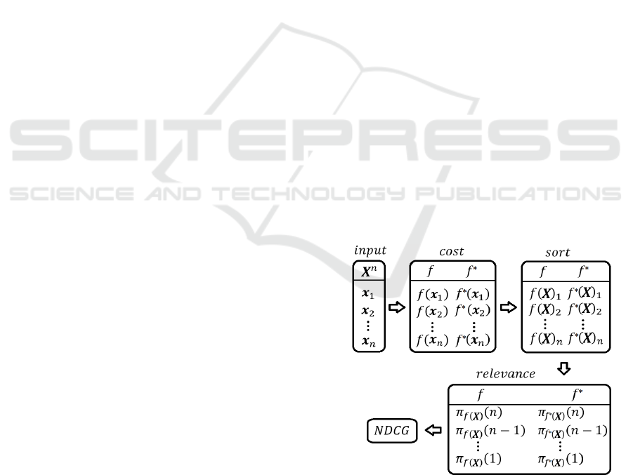
APPENDIX
NDCG flowchart: The below example shows how
Normalized Discounted Cumulative Gain (NDCG)
can be computed from input permutations (products
to locations), approximated (𝑓) and ground truth (𝑓
∗
)
values. Note that 𝑓
(
𝑿
)
denotes a sorting of 𝑿
according to the cost valuation of elements in the cost
step. Also note that relevance values can be
formulated in several ways.
Figure 4: NDCG flowchart.
IN4PL 2022 - 3rd International Conference on Innovative Intelligent Industrial Production and Logistics
34

Table 1: Summary of instances and results for the CPU-times of the OBP model (SBI) and the QAP model, as well as an
aggregate of the results concerning the predictive strength of the QAP model.
New Benchmarks and Optimization Model for the Storage Location Assignment Problem
35
