MLP-Supported Mathematical Optimization of Simulation Models:

Investigation into the Approximation of Black Box Functions of Any

Simulation Model with MLPs with the Aim of Functional Analysis

Bastian Stollfuss

1,2

and Michael Bacher

University Stuttgart, Stuttgart, Germany

University of Applied Science, Kempten, Germany

Keywords: Machine Learning, Supervised Learning by Regression, Mathematical Analysis, Approximation, Material

Flow Simulation, Process Optimization, Artificial Neuronal Network, Newton’s Method.

Abstract: This paper contains results from a feasibility study. The optimization of manufacturing processes is an

elementary part of economic thinking and acting. In many cases, complex processes have unknown analytical

and mathematical methods. If mathematical functions for the behaviour of a process are missing, one often

tries to optimize the process according to the trial-and-error principle in combination with expertise. However,

this method requires a lot of time, computational resources, and trained personnel to validate the results. The

method developed below can significantly reduce these cost factors by mathematically optimizing the

unknown functions of a complex system in an automatic process. This is accomplished with discrete

performance and behaviour measurements. For this purpose, an approximate prediction function is modelled

using a multi-layer perceptron (MLP). The resulting continuous function can now be analysed with

mathematical optimization methods. After formulating the learned prediction function, it is examined for

minima using Newton’s method. It is not necessary to know the exact mathematical and physical context of

the system that needs improving. Calculating a precise interpolation also results in further optimization and

visualization options for the production plant.

1 INTRODUCTION

The modern-day possibilities of digitization mean

that given processes are not simply adopted, but also

optimized. Especially in information technology and

business informatics, process or data mining, data

science, process management, artificial intelligence

(AI) are implemented as a matter of course (Laue et

al. 2021), (Li Zheng, Chunqiu Zeng, Lei Li, Yexi

Jiang, Wei Xue, Jingxuan Li, Chao Shen, Wubai

Zhou, Hongtai Li, Liang Tang, Tao Li, Bing Duan,

Ming Lei, Pengnian Wang 2014). Data-driven

process optimization is a huge topic of industry 4.0

(Paasche und Groppe 2022). This paper concerns the

feasibility of a new method of data-driven process

optimization.

If mathematical functions for the description of a

process are missing, one often tries to optimize the

process according to the archaic trial and error

principle (Bei et al. 2013).

When optimizing the simulation models, which

involved expert knowledge, empirical values and trial

and error in combination with expertise were mainly

used. The methodology is inefficient because of the

missing explanation component, which is replaced by

manual documentation and the associated high time

duration and human resources. This approach offers

opportunities for optimization by approximating the

discrete black box function of the simulation model

through a continuous function. Plant simulations do

not generate a continuous function, which would be

necessary for further mathematical processing (Rubin

et al. 1993).

We have to find a continuous approximation

function with an effective optimization and

subsequent return of the found results to the

simulation model.

The state of the art and the theory building of this

paper are summered in chapter 1. Chapter 2 covers

the system developed including plant simulation,

designing an MLP, definition of validation

parameters, training of the MLP, mathematical

Stollfuss, B. and Bacher, M.

MLP-Supported Mathematical Optimization of Simulation Models: Investigation into the Approximation of Black Box Functions of Any Simulation Model with MLPs with the Aim of Functional

Analysis.

DOI: 10.5220/0011379800003329

In Proceedings of the 3rd International Conference on Innovative Intelligent Industrial Production and Logistics (IN4PL 2022), pages 107-114

ISBN: 978-989-758-612-5; ISSN: 2184-9285

107

optimization. Chapter 3 contains the evaluation of the

developed system. Chapter 4 is discussing the

research results. The following chapter 5 gives a

Summary of our results. Finally, chapter 6 gives an

insight into the future research perspectives.

1.1 State of the Art

The topics of the optimization methods, which are

presented in the publications discussed, are artificial

neural network (ANN), Support Vector Regression

(SVR), Immune Particle Swarm Optimization

(IPSO), multi-layer perceptron (MLP), mathematical

optimization (MO), autoregressive integrated moving

average (ARIMA), evolutionary algorithm (EA).

The Paper (Yan Wang, Juexin Wang, Wei Du,

Chen Zhang, Yu Zhang, Chunguang Zhou 2009) is

about the downstream optimization of the SVR

learning method with the help of IPSO. It's about

improving hyperparameters of the SVR. In this work

the hyperparameter setting of the SVR is optimized

via IPSO.

The authors in (Andrei Solomon 2011) use

different prediction models, including ARIMA and

linear regression on time series, to improve the

simulation process parameters.

In (Ankur Sinha, Pekka Malo, Peng Xu,

Kalyanmoy Deb 2014), like SVR, hyperparameters

should be optimized. It's not about optimizing the

result, but about optimizing the hyperparameters for

a machine learning process. Bilevel optimization is a

special kind of programming in which an

optimization problem is embedded in an outer and

inner optimization problem, with an upper and lower

bound on the boundary conditions.

Generic algorithms are special optimization

methods in the field of evolutionary algorithms. The

publication (Nadir Mahammed, Souad Bennabi,

Mahmoud Fahsi 2020) deals with the optimization of

a business model design by Genetic Algorithm based

on multiple populations. Based on the business model

design, a mathematical representation is created and

fed into the optimization process. Starting with an

initial population, descendants are selected with the

help of an evaluation function and subsequent

selection. The selected offspring are modified and

entered into the original population. A new

population is obtained as the return value of the

evaluation function, which is processed in the same

way. The result is optimally parameterized business

process. Business process parameters have been

improved and greater diversity has been achieved.

Basically, the trial-and-error process is developed

further here because the random factor is preserved.

(B. Cavallo, M. D. Penta, and G. Canfora 2010) is

about an empirical study to reliably predict Quality of

Service (QoS). Various prediction models are used

for this, as Andrei Solomon in (Andrei Solomon

2011) ARIMA was also used here. For further

information see (Box 2015).

From the data generated in an industrial process,

the parameters are analysed with the help of data

mining (Li Zheng, Chunqiu Zeng, Lei Li, Yexi Jiang,

Wei Xue, Jingxuan Li, Chao Shen, Wubai Zhou,

Hongtai Li, Liang Tang, Tao Li, Bing Duan, Ming

Lei, Pengnian Wang 2014). The results are analysed

and processed, and the process parameters are

optimized using possibility theory and linear

regression.

In the publication (Zhaoxia Chen, Bailin He, and

Xianfeng Xu 2011), an ANN with backpropagation

(BP) is used directly to optimize processes. The data

is generated by a measuring stand. The structure of

the ANN is not analysed in detail, but the ANN

outputs the control parameters for the machine

directly. So direct error minimization takes place via

the ANN and BP.

Mathematical optimization is also a discipline of

applied mathematics. Like analytics, it is about

finding optimal parameters in a system so that a target

function can be minimized or maximized. An

analytical solution of optimization problems is often

not possible or too time-consuming and could be

replaced or supplemented by numerical methods.

However, the mathematical function to be analysed is

often unknown. Optimization is therefore also a

problem of approximation, which involves

minimizing the distance between two functions in

order to then process the function further (Alpaydın

2019).

In the method developed by the mining engineer

D. G. Kriging, a solution to the specific problem is

described, which determines promising locations for

further drilling sites with increased ore deposits based

on previous drilling sites. To achieve this, he

designed a method that became known as the Kriging

method or Gaussian Process Regression and thus

developed one of the first machine learning methods.

It is still used today when a function is to be

maximized for which an evaluation of the function

parameters is very complex and whose mathematical

derivations are not available (JARRE und Stoer

2019).

Because process optimization is a ‘black box

problem’, the use of ANN is suitable. The process

optimization creates large amounts of data from

which information is to be extracted, taking the black

box system into account. By training the ANN with

IN4PL 2022 - 3rd International Conference on Innovative Intelligent Industrial Production and Logistics

108

the discrete output values, we get a prediction

function. The weights are adjusted by the

backpropagation algorithm. We use the method

similar to the Gaussian process to solve a regression

problem. In our case, we use MLP for the following

task. The production times or cycle times represent

the output values depending on the input parameters

of the prediction function.

1.2 Hypothesis

The hypothesis of this study concerned whether an

MLP is able to approximate an unknown function

with sufficient accuracy in order to be able to draw

conclusions as to where the minima or maxima of this

unknown function are located.

1.3 Objective

The aim was to test an optimization method that uses

MLP to approximate functions in order to then

examine the prediction function for optima. The

optima found should be validated by returning them

to the simulation model. Furthermore, it should be

examined whether this method is better suited than

trial and error methods.

2 METHODS

2.1 Summary

Production plants can be simulated as a Blackbox

function with the input parameters A and B and the

output C, as cited below. C needs to be optimized

with the input parameters A and B. MLPs are able to

carry out universal approximations of Blackbox

functions (Alpaydın 2019). In our case the MLP

should now approximate the unknown function of the

simulation of a production plant. The resulting

prediction function is known in its entirety and can be

MO. Specifically, the goal is that after the learning

process, the MLP should behave exactly like the

simulation. The MLP used is extended by a special

activation function. Based on Fourier, the sine

function is used instead of the frequently used

sigmoid function (Egger 2006). The backpropagation

algorithm and Newton’s method can be easily

implemented through the simple symbolic derivation

of the sine function.

After successful training of the MLP, the

determined weights of the connections are saved.

With the known structure and the stored weights of

the MLP, the prediction function is formulated by a

self-implemented program. The prediction function

built in this way results in C´ depending on A and B.

C´ approximates C. C´ is now to be mathematically

optimized depending on A and B using the Newton

method. The parameters A and B can be determined

by the found minima of C´. The quality of the

prediction function can be verified by directly

comparing the Blackbox function output C with the

prediction function output C´. The MO works

automatically, apart from the hyperparameter

settings.

2.2 Simulation

The feasibility of the process described above is to be

proven and analysed using a material flow simulation.

A production plant should be optimized regarding its

cycle time. For this purpose, concrete data sets of this

production plant were first generated with a material

flow simulation.

Figure 1: Production plant.

The data records created contained the variable

parameters: workpiece carriers in the system and

permitted simultaneous number of workpiece carriers

in a part of the system (Sub Area), shown in Figure 1.

The training data generated by the simulation model

were discrete data pairs, which were then used for the

supervised learning of the MLP. The data were

automatically generated and mapped a combinatorial

grid over the area of interest.

The area of definition of the black box function to

be examined is the area in which a minimum is

assumed or an area that is determined by external

specifications and limitations. The simulation

calculated an output data structure containing the

cycle times with which the finished workpieces left

the system (Table 1).

MLP-Supported Mathematical Optimization of Simulation Models: Investigation into the Approximation of Black Box Functions of Any

Simulation Model with MLPs with the Aim of Functional Analysis

109

Table 1: Output data.

Workpiece

carriers

Produced

Workpieces

Workpiece

carriers in

sub-area

Average

cycle

time [s]

94 1000 5 707.4768

94 1000 6 688.9963

94 1000 7 682.2486

94 1000 8 671.8879

94 1000 9 670.1345

The structure of the output data is formed as a grid

area. The cycle time must be minimized by correctly

setting the variable parameters to improve the overall

productivity of the system. A prediction function is

now formulated from the MLP so that it can be

mathematically optimized.

2.3 Modified MLP

For this purpose, an MLP was created to train the data

sets, in this case the cycle time depending on the

variable system parameters. The MLP used was

expanded to include the sine function as an activation

function as shown in Figure 2, with amplitude a,

angular frequency ω and phase ϕ. Since the cosine

function is only phase-shifted, it is also described

(Papula 2014).

Figure 2: Illustration of the network structure with modified

activation function.

The property of a simple derivation of the sine or

cosine function forms the basis for the idea of using

this as an activation function. Since the weights

should not diverge or convert to zero during the

learning process, the input and output values were

normalized beforehand. The backpropagation

algorithm was used to adjust the weights in the

learning process. Depending on the previous weights,

this propagates the error back and adjusts the current

weights according to their influence.

2.4 Validation

Various error parameters were calculated to evaluate

the quality of the prediction function, including

RMSE, MAE and



(Alpaydın 2019).

Since this is a new activation function that cannot

be set in the usual libraries, the MLP was self-

implemented. Known functions for determining the

quality of the MLP were used to test the created

program code for correct functionality. The first test

runs took place with random well-known (Eq. 1., Eq.

2), two-dimensional functions. Once these could be

approximated very well after setting the

hyperparameters, the test was extended to three-

dimensional functions, which also has been

successfully approximated.

2.4.1 2D-Function





120

(1)

Figure 3: Original function (left) and funtion approximation

(right).

Table 2: Results of test run with 2d function.

och RMSE MAE R2

198 0.287285 0.215675 0.999898

2.4.2 3D-Function





x⋅y

ⅇ





(2)

Figure 4: Original function (left) and function

approximation (right).

The pairwise-compared functions, original function

and approximation agree in a self-defined quality

criterion up to 2% MAE. (Figure. 3,4) and Table 2,

Table 3.

IN4PL 2022 - 3rd International Conference on Innovative Intelligent Industrial Production and Logistics

110

Table 3: Results of test run with 3d function.

Epoch RMSE MAE R2

19 1.192364 0.780794 0.998744

2.5 Training

The data set generated by the simulation contains

about 650 labelled data (Fig. 5). After successful

online learning, the MLP can predict the cycle time

with a corresponding level of accuracy, which can be

found in Table 4.

Figure 5: Plot of the data set calculated by the simulation

model.

Figure 6: Approximation of the data set by ANN4.

The prediction function of the fully trained MLP,

which is shown in Fig. 6, was now used to find the

minima of the cycle time. The prediction function was

extracted using a program designed for this purpose.

The number of summed and nested sine functions is

defined by the structure of the MLP. The learned

weights were each inserted as a factor in front of the

individual sine functions. Since the nesting and the

summation always follow the same pattern, this

surrogate function was created in different “for-

loops”. At the end of the algorithm, the finished

prediction function was outputted.

Table 4: Results of the MLP training.

MLP: Epoch RMSE MAE

𝑅



MLP1 904 0.069216 0.054091 0.834757

MLP2 312 0.055734 0.047214 0.883755

MLP3 21815 0.053844 0.044480 0.830314

MLP4 7803 0.041716 0.034093 0.941049

For the purpose of mathematically optimizing the

prediction function, minima were now sought in the

area shown in Table 5. The definition area of the

prediction function (Fig. 6) consists of the limited

ranges of the input parameters. The range of

parameters to be examined was between 20 100

workpiece carriers in the entire system and 5 20

workpiece carriers in the limited sub-area of the

system (Fig. 1).

Table 5: Limits of the generated data set.

Workpiece

carriers [n]

Workpiece

carriers in

sub-area[n]

Average

cycle

time [s]

Lower limit 20 5 640.64

Upper limit 100 20 862.65

Increment 2 1

2.6 Mathematical Optimization

The Newton method as an iteration method is very

well suited to finding extreme points. For this

purpose, the first and second partial derivatives of the

prediction function were formed first. Since the

prediction function only consists of nested and

weighted sine functions, it can be derived simply

symbolically, and a numerical derivation is not

necessary. This avoids rounding errors and

discretization errors. The second partial derivatives

MLP-Supported Mathematical Optimization of Simulation Models: Investigation into the Approximation of Black Box Functions of Any

Simulation Model with MLPs with the Aim of Functional Analysis

111

were assembled into the Jacobian matrix, which is

used in the so-called Newton step to determine the

local gradient of the prediction function. Since there

are multidimensional extreme points, it must be

checked whether each extremum is a minimum in all

dimensions by using the Jacobian matrix.

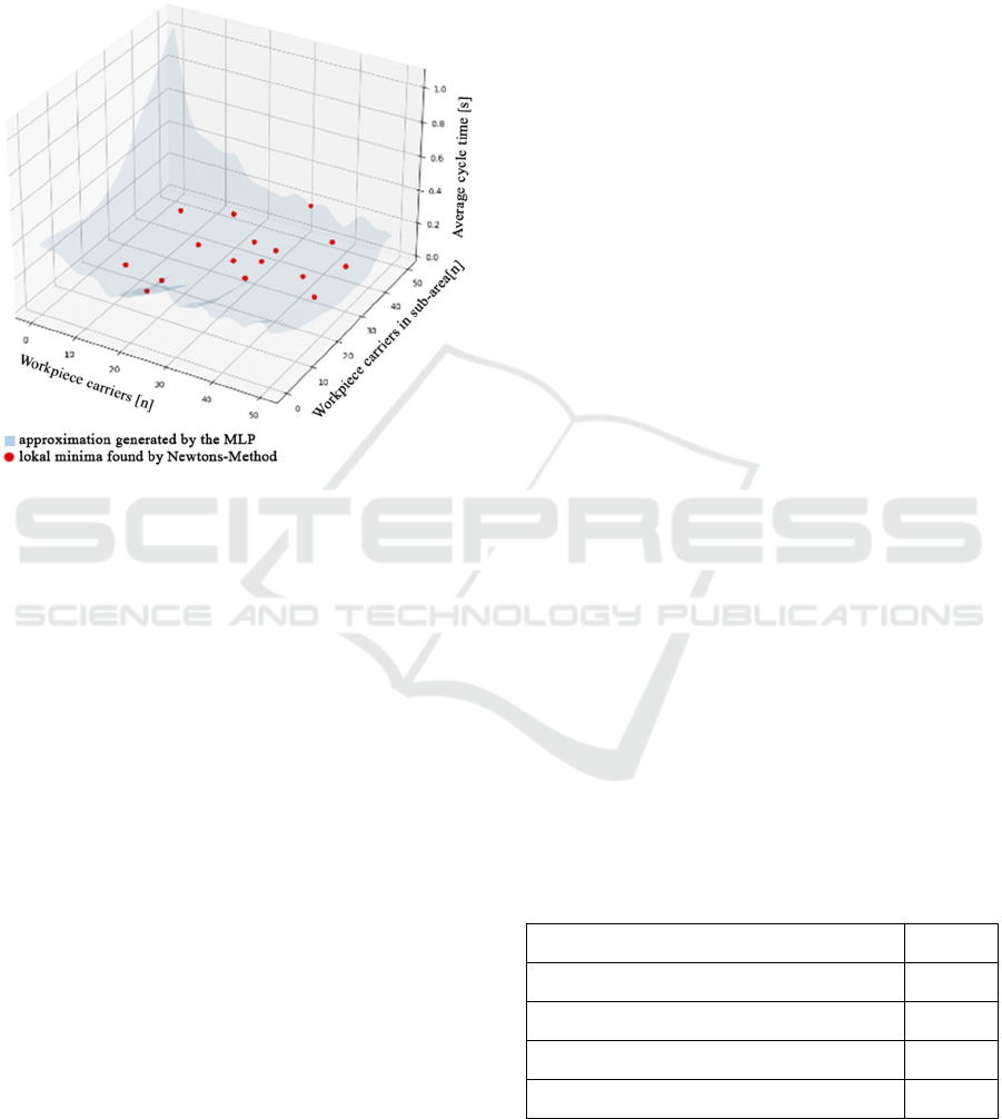
Figure 7: Approximation by MLP3P4 and identified

minima.

A starting point in the definition area is first

defined in the Newton´s method, after which several

Newton steps are carried out from this starting point.

The starting point can converge to a local minimum.

If the starting point diverges, the program aborts after

a certain number of Newton steps. In order to find as

many local minima as possible in the target area, a

combinatorial grid out of the definition area with the

required resolution of starting points was created.

Now local minima of the cycle time and their

responsible parameters in the prediction function

could be determined using the Newton method

(Figure 7).

The parameters of the calculated local minima

were converted to inverse the normalization that was

initially introduced. Then, the parameters found,

which lead to a minimum of the cycle time were

entered into the simulation for evaluation. Finally, it

was checked whether a shorter cycle time was

achieved with the calculated parameters.

3 EVALUATION

As a result, it was possible to train the MLP in such a

way that the cycle time of the plant could be predicted

with a high degree of certainty (Table 4). The

function of the best MLP approximates the behaviour

of the simulation model regarding the cycle time with

a coefficient of determination R

up to 0.94. The mean

absolute error corresponded to about 7.56 seconds out

of an average of 686.63 seconds for the cycle time

(1.1%). The result is better than the deviation of 2%

determined with the test functions in section 2.4.

After successfully training and extracting the

prediction function, it could be visualized as a

continuum. Checking the found minima provides

certainty, and the procedure does not require human

assistance, but works automatically.

If the predicted minima were greater than the

values calculated by the simulation, they were

classified as incorrect. The incorrectly predicted

minima could be traced back to interpolation

inaccuracies. The global minimum was determined

by paired comparison of all local minima. In four of

the 16 MLPs examined, an improvement in the cycle

time was achieved due to mathematical optimization.

The data set for all 16 MLPs examined includes

around 10,000 label data. In order to compare the

mathematically optimized procedure with the trial-

and-error method, randomly selected parameter

combinations were entered manually, and the results

collated to a test suite.

Collecting the data from the trial-and-error

method should take about as long as the procedure of

the developed algorithm.

For this purpose, the time required for training the

MLP and mathematical optimization was calculated,

as shown in Table 6.

For the benchmark of the MLP and MO versus

trial and error, both processes are given 6 hours to

find the global minimum of the cycle time. The trial-

and-error test suite mentioned above was generated in

6 hours by hand. In contrast to the trial-and-error

procedure, training the MLP by hand only takes 2

hours, thus saving 4 man-hours.

Table 6: Duration time.

650 data generated automatically 1.5 h

Training 2 h

Determining minima and global minimum 2 h

Other steps of procedure 0.5 h

Sum 6 h

The data set comprised 500 data pairs (Fig. 8).

Due to the manual input of the parameters and the

aimless generation of data, the data record is shorter

IN4PL 2022 - 3rd International Conference on Innovative Intelligent Industrial Production and Logistics

112

than the automatically generated data record. In

addition, it is not as evenly distributed over the

definition area, while the MLP dataset is discrete.

The global minimum in this dataset is 646,78s.

The global minimum determined by trial and error is

5.12s worse than the minimum time determined by

the MLP and the mathematical optimization, shown

in Table 7.

Figure 8: Test suite.

Table 7: Results.

Process Global

Minimum

[s]

Workpiece

carrier

[n]

Workpiece

carrier in

sub-area

[n]

MLP and

mathematical

optimization

641.66 100 17

Trial and

error in Plant

Simulation

646.78 92 15

4 DISCUSSION

Process optimization of complex manufacturing

systems, which is used in many production plants, is

often difficult and confusing in practice, since the

mathematical and physical relationships of the factors

influencing the system are not known, resulting in a

black box function.

Finding suitable hyperparameters for the

respective learning task is sometimes very time-

consuming. However, once hyperparameters were

found, they could be used again and again for the

application. The time required to train the MLP was

2 hours, on average, requiring no further work steps

by hand. However, the calculation time was

dependent on external factors, such as the number of

input data, size of the MLP, number of epochs,

performance of the source code, and the performance

of the computing components. Overall, however, very

good automation of the process was possible.

Furthermore, only short, wide MLPs could be

evaluated, as the gradient calculation for long, narrow

MLPs is significantly more complex. The reason for

this lies in the partial derivatives for the gradient

method, which are calculated symbolically. The

extracted function is a nesting of the transfer and

activation function. Thus, the need for post-

differentiation increases exponentially with each

additional layer.

5 SUMMARY

Training an MLP with a complex black box function

has proven to be feasible. In some cases, a cycle time

advantage of the MLP and MO procedure compared

to the trial-and-error method could also be shown.

This benefit is tied to its definition area. This means

that the global minimum is outside of our definition

area. In this case it is only a local minimum inside the

definition area. However, the definition range was

realistic from a technical point of view. For example,

it is not possible to feed any number of workpiece

carriers into a limited conveyor belt section, even if

this would result in infinitely short cycle times.

The process can be automated in the main and, in

the case of complex problems, is faster than the trial-

and-error method due to the reduction in manual

work. This results in a productivity advantage

through the saving of human resources. With the

method using MLPs and MO, it is not necessary to

know the exact mathematical and physical

relationships of the Blackbox system to be improved.

6 PERSPECTIVE

The MLP and MO procedure can also be applied to

other functions. In this way, functions could be

predicted for which there are no simulation models.

In this case, a test stand forms the basis from which

empirically discrete data can be obtained, but the

exact mathematical function behind the system is

unknown. With the help of base values, a prediction

function is interpolated with MLPs. The subject of a

MLP-Supported Mathematical Optimization of Simulation Models: Investigation into the Approximation of Black Box Functions of Any

Simulation Model with MLPs with the Aim of Functional Analysis

113

further publication could be a performance evaluation

and comparison between the MLP and MO procedure

and the trial-and-error procedure on a simulation

model.

REFERENCES

Alpaydın, Ethem (2019): Maschinelles Lernen. 2. Auflage.

Berlin, Boston: De Gruyter (De Gruyter Studium).

Andrei Solomon, Marin Litoiu (2011): Business Process

Performance Prediction on a Tracked Simulation

Model. In: Manuel Carro (Hg.): Proceedings of the 3rd

International Workshop on Principles of Engineering

Service-Oriented Systems. New York, NY: ACM

(ACM Conferences), S. 50–56.

Ankur Sinha, Pekka Malo, Peng Xu, Kalyanmoy Deb

(2014): A Bilevel Optimization Approach to

Automated Parameter Tuning. In: Proceedings and

companion publication of the 2014 Genetic and

Evolutionary Computation Conference, July 12 - 16,

2014, Vancouver, BC, Canada ; a recombination of the

23rd International Conference on Genetic Algorithms

(ICGA) and the 19th Annual Genetic Programming

Conference (GP) ; one conference - many mini-

conferences ; [and co-located workshops proceedings].

New York, NY: ACM, S. 847–854.

B. Cavallo, M. D. Penta, and G. Canfora (2010): An

empirical comparison of methods to support QoS-

aware service selection. In: Grace A. Lewis (Hg.):

Proceedings of the 2nd International Workshop on

Principles of Engineering Service-Oriented Systems.

New York, NY: ACM (ACM Conferences), S. 64–70.

Bei, Xiaohui; Chen, Ning; Zhang, Shengyu (2013): On the

complexity of trial and error. In: Dan Boneh, Tim

Roughgarden und Joan Feigenbaum (Hg.): Proceedings

of the 45th annual ACM symposium on Symposium on

theory of computing - STOC '13. the 45th annual ACM

symposium. Palo Alto, California, USA, 01.06.2013 -

04.06.2013. New York, New York, USA: ACM Press,

S. 31.

Box, George E. P. (2015): Time Series Analysis.

Forecasting and Control. 5th ed. Hoboken: Wiley

(Wiley Series in Probability and Statistics).

Egger, Dieter (2006): Sinus-Netzwerk. In: TU München:

Schriftenreihe des Instituts für Astronomische und

Physikalische Geodäsie und der Forschungseinrichtung

Satellitengeodäsie 22.

Jarre, Florian; Stoer, Josef (2019): Optimierung.

Einführung in mathematische Theorie und Methoden.

2. Auflage. Berlin, Heidelberg: Springer Spektrum

(Masterclass).

Laue, Ralf; Koschmider, Agnes; Fahland, Dirk (Hg.)

(2021): Prozessmanagement und Process-Mining.

Grundlagen. Berlin/München/Boston: Walter de

Gruyter GmbH (De Gruyter Studium Ser). Online

verfügbar unter https://ebookcentral.proquest.com/lib/

kxp/detail.action?docID=5156279.

Li Zheng, Chunqiu Zeng, Lei Li, Yexi Jiang, Wei Xue,

Jingxuan Li, Chao Shen, Wubai Zhou, Hongtai Li,

Liang Tang, Tao Li, Bing Duan, Ming Lei, Pengnian

Wang (2014): Applying Data Mining Techniques to

Address Critical Process Optimization Needs in

Advanced Manufacturing. In: Proceedings of the 20th

ACM SIGKDD International Conference on

Knowledge Discovery and Data Mining, August 24 -

27, 2014, New York, NY, USA. New York, NY: ACM,

S. 1739–1748.

Nadir Mahammed, Souad Bennabi, Mahmoud Fahsi

(2020): Optimizing Business Process Designs with a

Multiple Population Genetic Algorithm. In: Richard

Chbeir (Hg.): Proceedings of the 10th International

Conference on Web Intelligence, Mining and

Semantics. New York, NY,United States: Association

for Computing Machinery (ACM Digital Library), S.

252–254.

Paasche, Simon; Groppe, Sven (2022): Enhancing data

quality and process optimization for smart

manufacturing lines in industry 4.0 scenarios. In: Sven

Groppe, Le Gruenwald und Ching-Hsien Hsu (Hg.):

Proceedings of The International Workshop on Big

Data in Emergent Distributed Environments.

SIGMOD/PODS '22: International Conference on

Management of Data. Philadelphia Pennsylvania, 12 06

2022 12 06 2022. New York, NY, USA: ACM, S. 1–7.

Papula, Lothar (2014): Mathematik für Ingenieure und

Naturwissenschaftler. 14., überarb. und erw. Aufl.

Erscheinungsort nicht ermittelbar (Mathematik für

Ingenieure und Naturwissenschaftler).

Rubin, Stuart H.; Fogel, David; Hanson, John C.; Kick,

Russell; Malki, Heidar A.; Sigwart, Charles et al.

(1993): The impact of machine learning on expert

systems. In: Stan C. Kwasny und John F. Buck (Hg.):

Proceedings of the 1993 ACM conference on Computer

science - CSC '93. the 1993 ACM conference.

Indianapolis, Indiana, United States, 16.02.1993 -

18.02.1993. New York, New York, USA: ACM Press,

S. 522–527.

Yan Wang, Juexin Wang, Wei Du, Chen Zhang, Yu Zhang,

Chunguang Zhou (2009): Parameters Optimization of

Support Vector Regression Based on Immune Particle

Swarm Optimization Algorithm. In: 2009 World

Summit on Genetic and Evolutionary Computation.

2009 GEC Summit; June 12 - 14, 2009, Shanghai,

China. New York, NY: ACM Press, S. 997–1000.

Zhaoxia Chen, Bailin He, and Xianfeng Xu (2011):

Application of Improved BP Neural Network in

Controlling the Constant-Force Grinding Feed. In:

Computer and computing technologies in agriculture

IV. 4th IFIP TC 12 conference, CCTA 2010, Nanchang,

China, October 22-25, 2010; selected papers.

Heidelberg: SPRINGER (IFIP advances in information

and communication technology, 347), S. 63–70.

IN4PL 2022 - 3rd International Conference on Innovative Intelligent Industrial Production and Logistics

114