Towards View-invariant Vehicle Speed Detection from Driving Simulator

Images

Antonio Hern

andez Mart

ınez

1 a

, David Fern

andez Llorca

1,2 b

and Iv

an Garc

ıa Daza

1 c

Computer Engineering Department, University of Alcal

a, Alcal

a de Henares, Spain

European Commission, Joint Research Centre (JRC), Seville, Spain

Keywords:

Vehicle Speed Detection, Driving Simulator, CARLA, View-invariant, Multi-view, Speed Camera.

Abstract:

The use of cameras for vehicle speed measurement is much more cost effective compared to other technologies

such as inductive loops, radar or laser. However, accurate speed measurement remains a challenge due to

the inherent limitations of cameras to provide accurate range estimates. In addition, classical vision-based

methods are very sensitive to extrinsic calibration between the camera and the road. In this context, the use of

data-driven approaches appears as an interesting alternative. However, data collection requires a complex and

costly setup to record videos under real trafﬁc conditions from the camera synchronized with a high-precision

speed sensor to generate the ground truth speed values. It has recently been demonstrated (Martinez et al.,

2021) that the use of driving simulators (e.g., CARLA) can serve as a robust alternative for generating large

synthetic datasets to enable the application of deep learning techniques for vehicle speed estimation for a

single camera. In this paper, we study the same problem using multiple cameras in different virtual locations

and with different extrinsic parameters. We address the question of whether complex 3D-CNN architectures

are capable of implicitly learning view-invariant speeds using a single model, or whether view-speciﬁc models

are more appropriate. The results are very promising as they show that a single model with data from multiple

views reports even better accuracy than camera-speciﬁc models, paving the way towards a view-invariant

vehicle speed measurement system.

1 INTRODUCTION

A clear causal relationship between excess speed and

the risk of death and serious injury is well-established.

Thus, speed enforcement through automatic speed

measurement, vehicle identiﬁcation and subsequent

sanctioning is a fundamental road safety measure that

leads directly to the reduction of accidents (ERSO,

EC, 2018). In fact, in the vicinity of speed cameras,

the reduction of speeding vehicles and collisions can

reach 35% and 25% respectively (Wilson et al., 2010).

In addition, it has been shown that the higher the in-

tensity of the enforcement, the greater the reduction

in accidents (Elvik, 2011).

Most common speed measurement technologies

include high-accuracy, high-cost range sensors such

as radar and laser, as well as intrusive sensors such

as magnetic inductive loop detectors. The use of

https://orcid.org/0000-0001-5722-1531

https://orcid.org/0000-0003-2433-7110

https://orcid.org/0000-0001-8940-6434

cameras has rarely been proposed for speed detec-

tion due to the demanding requirements for accuracy

and robustness, and the intrinsic limitations of cam-

eras to accurately measure range. They often play

a secondary role in detecting license plates or cap-

turing human-understandable information from the

scene, allowing visual identiﬁcation of vehicles, even

drivers, and serving as evidence when the speed limit

is violated. Recent advances in computer vision, how-

ever, have led to a signiﬁcant increase in the number

of proposals that use vision as the only mechanism

for measuring vehicle speed (Fern

andez-Llorca et al.,

2021). Cameras are a very cost-effective alternative

that allows the integrated implementation of speed

detection along with other functionalities such as li-

cense plate detection, automatic vehicle identiﬁcation

or even occupant detection.

188

Martínez, A., Llorca, D. and Daza, I.

Towards View-invariant Vehicle Speed Detection from Driving Simulator Images.

DOI: 10.5220/0011380000003335

In Proceedings of the 14th International Joint Conference on Knowledge Discovery, Knowledge Engineering and Knowledge Management (IC3K 2022) - Volume 1: KDIR, pages 188-195

ISBN: 978-989-758-614-9; ISSN: 2184-3228

Camera Settings

Environment

Vehicle

Camera Pose 1

Camera Pose 2

Camera Pose N

3D CNN 1

Camera Pose 1

3D CNN 2

3D CNN N

3D CNN Holistic

Figure 1: Overview of the presented approach. From left to right: control parameters, simulator, camera-speciﬁc datasets,

view-speciﬁc models, and view invariant (holistic) model.

Still, vision-based speed measurement is a chal-

lenging problem due to the discrete nature of video

sensors. In addition, classical vision-based methods

are very sensitive to extrinsic calibration between the

camera and the road. In this context, the use of data-

driven approaches appears as an interesting alterna-

tive but real data collection requires a complex setup

(Llorca et al., 2016). It has recently been proved that

the use of driving simulators (e.g., CARLA) can serve

as a robust alternative for generating large synthetic

datasets to enable the application of deep learning

techniques for vehicle speed estimation from a single

camera (Martinez et al., 2021) or from multiple views

(Barros and Oliveira, 2021).

In this paper, we extend our previous work (Mar-

tinez et al., 2021) by addressing the question of

whether complex end-to-end 3D-CNN architectures

(i.e., regression problem, from sequences to speeds)

are capable of implicitly learning view-invariant

speeds using a single holistic model, or whether view-

speciﬁc models are more appropriate. We extend our

synthetic dataset based on CARLA simulator (Doso-

vitskiy et al., 2017) using six different virtual cam-

eras with variations in height and pitch angle. Then

six view-speciﬁc models are developed and compared

with one single multi-view model trained with se-

quences from all the cameras. An overall view of the

proposed approach is depicted in Fig. 1. The results

presented are very promising as they suggest that the

model is capable not only of absorbing the variability

of multiple views, but also of beneﬁting from it and

from the increased availability of data, which opens

the door to future view-invariant systems.

2 RELATED WORK

As the survey presented in (Fern

andez-Llorca et al.,

2021) concludes, although we can ﬁnd hundreds of

works focused on vision-based vehicle speed detec-

tion, the available solutions are not sufﬁciently ma-

ture. A considerable number of papers present sub-

optimal camera pose and settings resulting in very

high meter-to-pixel ratios that are unlikely to provide

accurate estimates of depth and speed. Performance

and robustness in difﬁcult lighting and weather condi-

tions are often neglected. The sensitivity of each ap-

proach to pose and camera settings is not sufﬁciently

addressed.

In addition, the number of data-driven approaches,

well consolidated in other areas of computer vision, is

still very limited for speed regression. This may also

be due to the lack of well-established datasets to train

and compare the performance of different methods. In

this section, we focus on recent learning-based meth-

ods for vision-based vehicle speed detection from the

infrastructure, including available datasets. We refer

to (Fern

andez-Llorca et al., 2021) for a more com-

plete overview of the state-of-the-art.

2.1 Learning-based Approaches

Regarding the estimation of vehicle speed using data-

driven methods, only a few papers are found in the

available literature. In (Dong et al., 2019), average

trafﬁc speed estimation is addressed as a video action

recognition problem using 3D CNNs. They concate-

nate RGB and optical ﬂow images and found that op-

tical ﬂow was more useful. They emphasize that the

main limitation is overﬁtting due to the lack of avail-

able data. In (Madhan et al., 2020) a Modular Neu-

ral Network (MNN) architecture is presented to per-

form joint vehicle type classiﬁcation and speed detec-

tion. These two approaches are more suitable for av-

erage trafﬁc speed detection, since the input data cor-

respond to multiple lanes and vehicles. Some kind of

mechanism is needed to generate regions of interests

with sufﬁcient spatio-temporal information (Biparva

et al., 2022) to distinguish different speeds for differ-

ent types of vehicles and scenarios. This issue can

Towards View-invariant Vehicle Speed Detection from Driving Simulator Images

189

be mitigated by using a camera setting with a lower

meter-pixel ratio focusing on a single lane.

Recent works have proposed the use of LSTM-

type recurrent architectures (Parimi and Jiang, 2021),

(Martinez et al., 2021), but as demonstrated in (Mar-

tinez et al., 2021) with synthetic data, they seem

to perform worse than other non-recurrent methods

such as 3D CNNs. In (Revaud and Humenberger,

2021) camera calibration, scene geometry and traf-

ﬁc speed detection are performed using a transformer

network in a learning process from synthetic training

data, considering that cars have similar and known 3D

shapes with normalized dimensions. In (Rodr

ıguez-

Rangel et al., 2022), after vehicle detection and track-

ing using YOLOv3 and Kalman ﬁlter, respectively,

a linear regression model is used to estimate the ve-

hicle speed. Other statistical and machine learning-

based methods are also compared. Vehicle detection

and tracking is performed in (Barros and Oliveira,

2021) using Faster R-CNN and DeepSORT, respec-

tively. Next, dense optical ﬂow is extracted using

FlowNet2, and ﬁnally, a modiﬁed VGG-16 deep net-

work is used to perform speed regression.

2.2 Datasets for Speed Detection

So far, only two datasets with real sequences and

ground truth values are publicly available. First, the

BrnoCompSpeed dataset (Sochor et al., 2017), which

contains 21 sequences (∼1 hour per sequence) with

1920 × 1080 pixels resolution images at 50 fps in

highway scenarios. The speed ground truth is ob-

tained using a laser-based light barrier system. Sec-

ond, the UTFPR dataset (Luvizon et al., 2017), which

includes 5 hours of sequences with 1920 × 1080 pix-

els resolution images at 30 fps in an urban scenario.

The ground truth speeds are obtained using inductive

loop detectors.

Therefore, as described above, the use of synthetic

datasets is becoming increasingly prevalent for this

problem. For example, in (Lee et al., 2019) a CNN

model to estimate the average speed of trafﬁc from

top-view images is trained using synthesized images,

which are generated using a cycle-consistent adver-

sarial network (Cycle-GAN). Synthetic scenes with

a resolution of 1024 × 768 pixels covering multiple

lanes with vehicles randomly placed on the road are

used in (Revaud and Humenberger, 2021) to train and

test the method used to jointly deal with camera cal-

ibration and speed detection. In our previous work

(Martinez et al., 2021), a publicly available synthetic

dataset was generated using CARLA simulator, us-

ing one ﬁxed camera at 80 FPS with Full HD format

(1920 ×1080), with variability corresponding to mul-

tiple speeds, different vehicle types and colors, and

lighting and weather conditions. A similar approach

was presented in (Barros and Oliveira, 2021) includ-

ing multiple cameras and generating more than 12K

instances of vehicles speeds. Preliminary, it is ob-

served that multi-camera variability does not nega-

tively affect the results. However, this effect has not

been sufﬁciently studied.

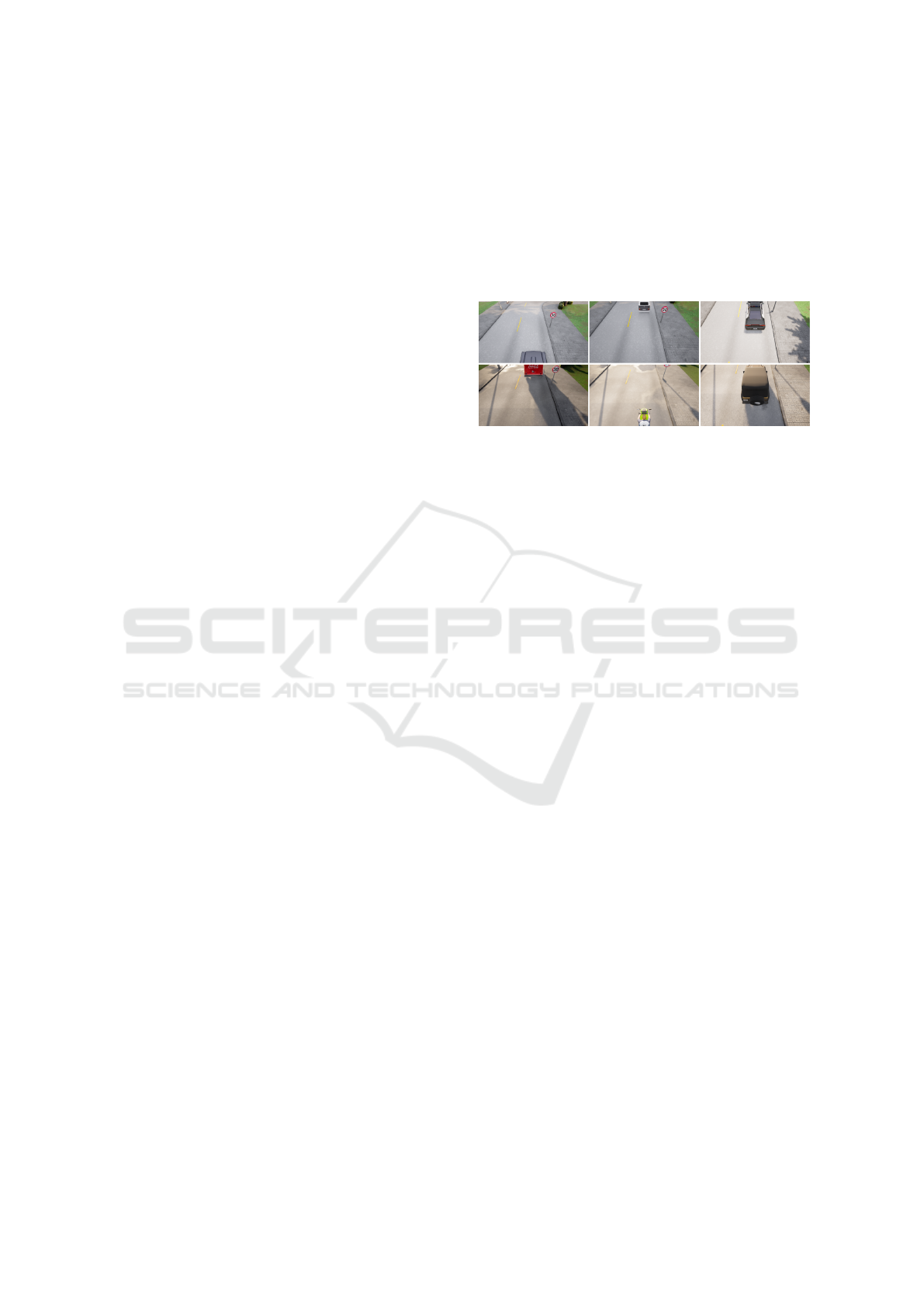
Figure 2: Overview of the different datasets. Upper row 4m

camera height. Lower row 3m camera height. The columns

show an 45º, 50º and 60º camera pitch from left to right.

3 METHOD

This section describes the methodology used for the

construction of the new dataset, based on the one

shown in the previous work (Martinez et al., 2021),

including new camera poses, and increasing the com-

plexity of the speed detection problem.

3.1 Multi-view Synthetic Dataset

Starting from the single-view synthetic dataset gen-

erated in the our previous work (Martinez et al.,

2021) using the CARLA simulator (Dosovitskiy et al.,

2017), the extrinsic parameters of the camera are

modiﬁed, speciﬁcally the pitch angle and the height

with respect to the road, leaving the rest of the extrin-

sic and intrinsic parameters ﬁxed.

As a ﬁrst step to increase variability in a controlled

manner and to be able to carry out a comprehensive

analysis of results, we included six different poses,

using two different camera heights and three different

pitch angles (extrinsic parameters): 3m45 (the origi-

nal one), 3m50, 3m60, 4m45, 4m50 and 4m60. On

the one hand, a holistic model is generated, trained,

validated and tested using all the sequences in the

dataset. On the other hand, pose-speciﬁc models are

trained, validated and tested only with the sequences

corresponding to each pose. Fig. 3 depicts how the

dataset is used.

For the selected camera heights (3m and 4m) the

three pitch angels have been deﬁned taking into ac-

count the road section captured by the camera ﬁeld

of view. For pitch angles greater than 60

◦

the road

section is too short, while for angles less than 45

◦

KDIR 2022 - 14th International Conference on Knowledge Discovery and Information Retrieval

190

Multi-pose camera dataset

3m45 *.json

images

3m50 *.json

images

4m60 *.json

images

3m45 model

3m50 model

4m60 model

Holistic

model

Figure 3: Schematic view of the dataset processing method.

the section is too long (for more details on the opti-

mal distances for speed detection see (Llorca et al.,

2016)). With these conﬁgurations, road sections of

between 4 and 10 meters in length were obtained.

Therefore, six camera poses were used, generating

610 sequences per pose (total number of sequences

is 3660). Each sequence with the associated vehi-

cle has a random speed between 30 and 100 km/h.

The sequence has an individual number of images de-

pending on the speed. Thus, the number of images

recorded in the dataset is approximately 427k. An ex-

ample image is shown in Fig. 2 for each camera pose.

Each simulation carried out to obtain the image se-

quences generates a json ﬁle. The json ﬁles record the

frame number, the brand and model of the simulated

vehicle, as well as its speed and ID, among other keys.

With the json ﬁle, and using the ID, the labelling can

be divided into sequences, each with the number of

frames generated depending on the vehicle speed.

To generate the labelling of the holistic model, the

json ﬁles of each of the simulations are combined,

adding for each sequence a new key indicating the

dataset from which the sequence comes. In this way,

each model can be evaluated individually, and cross

tests can also be performed, as in the case of the holis-

tic model, which has been used to test each of the

datasets.

Listing 1: json ﬁle labeling example.

1 {" elapsed seconds " :2.0 5 ,

2 " de l t a _ s ec o n d s " : 0 . 0 1 2 5 ,

3 " p l a t f o r m _ ti m e s ta m p " : 5 9 7 5 4 4 . 3 7 ,

4 " x " : 3 9 2 . 1 9 ,

5 " y " : 3 0 4 . 0 ,

6 " velocity " : 2 4 . 0 4 2 ,

7 " player_ i d " : 2 5 9 ,

8 " pl a y e r _ t y p e " : " vehicle .

car l a m o t o r s . c a r l a c o l a " ,

9 " attr i b u t e s " : {

10 " n u m b e r _ o f _ w he e l s " : " 4 " ,

11 " s t i c k y _ co n t r o l " : " t r ue " ,

12 " o b je c t _ t y p e " : "" ,

13 " c olor " : " 2 5 5 , 6 8 , 0 " ,

14 " r o l e _ name " : " hero "

15 },

16 " w eat h e r _ t y pe " : "

We a t h e r P a r a m e t e r s (

clou d i n e s s = 3 0 . 0 ,

pr e c i p i t a t i o n = 4 0 . 0 ,

pr e c i p i t a t i o n _ d e p o s i t s =4 0 .

0 , wi n d _ i n t e n s i t y = 3 0 . 0 ,

su n _ a z i m u t h _ a n g l e = 2 5 0 . 0 ,

su n _ a l t i t u d e _ a n g l e = 2 0 . 0 ,

fog _ d e n s i t y = 1 5 . 0 ,

fog _ d i s t a nc e = 5 0 . 0 ,

fog _ f a l l o f f = 0 . 9 , wetness = 8

0 . 0 ) "

17 }

Listing 1 shows one of the frames labeled in the

json ﬁle, where the aforementioned keys can be ob-

served. In addition, the time elapsed between two

consecutive images, the X and Y positions of the ve-

hicle, and the vehicle’s speed can be veriﬁed alterna-

tively with this data.

3.2 3D-CNN model

On this occasion, although the VGG16-GRU net-

work used previously (Martinez et al., 2021) obtained

highly successful results, it was decided to continue

with the use of the 3D-CNN network, since it showed

better performance.

Hence, in order to compare the different results

obtained in each training performed, it has been de-

cided not to modify any of the parameters or hyper-

parameters of the neural network.

First of all, it has been decided to perform an in-

dividual training for each of the mentioned datasets,

in this way it has been possible to check which of the

conﬁgurations used is better for the proposed system.

After this, it has been decided to perform a train-

ing on the complete dataset, with all the sequences of

each of the individual datasets, in order to check the

generalization capacity of the network.

Finally, this model trained with the complete set

of images has been tested with each of the test sets

of the different individual datasets. In order to per-

form this type of tests, it has been guaranteed that the

holistic model has not seen any of the test images of

the individual models in its training.

Towards View-invariant Vehicle Speed Detection from Driving Simulator Images

191

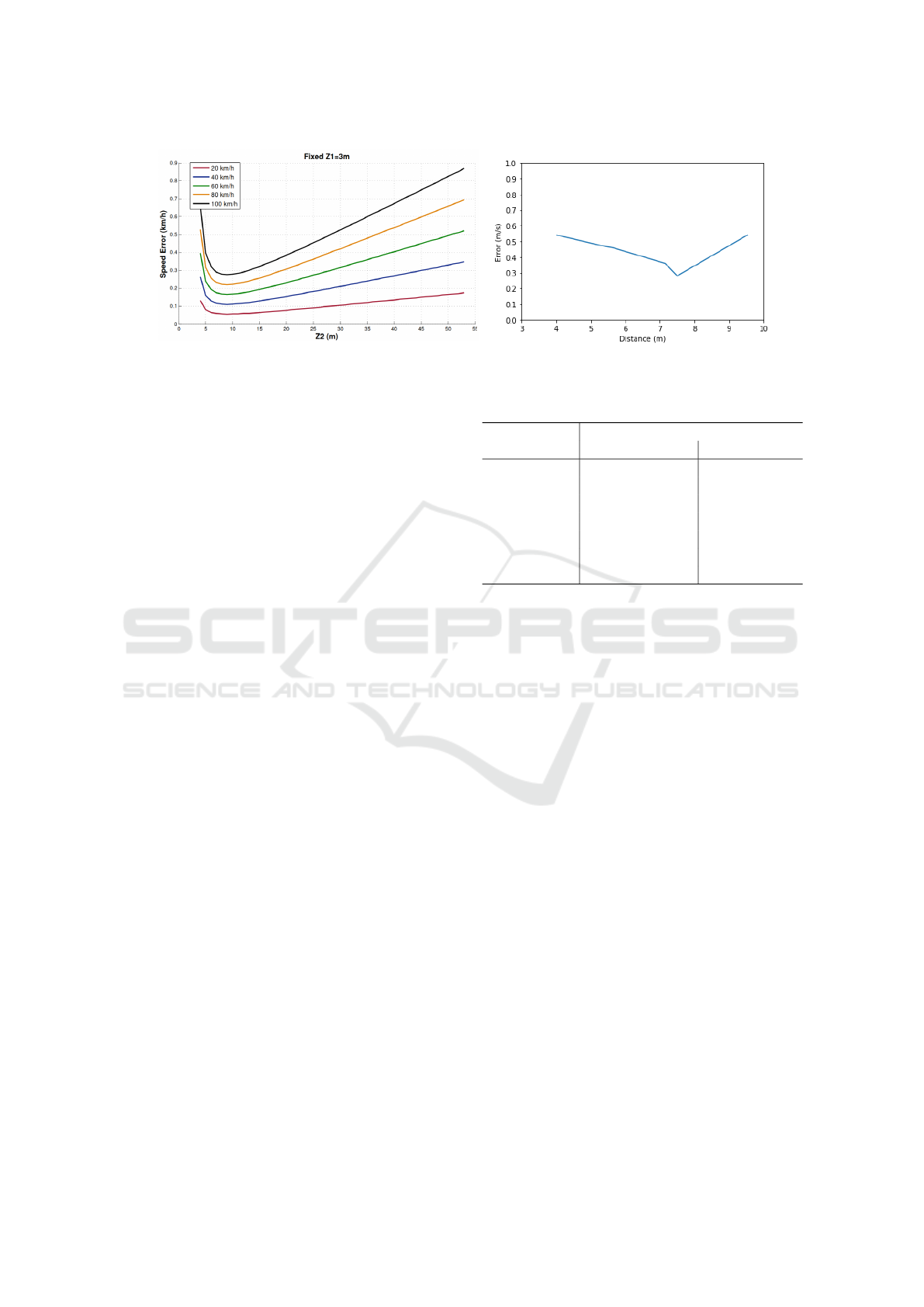
Figure 4: Left: theoretical speed estimation error with respect to the distance of the measurement section. From (Llorca et al.,

2016). Right: obtained results of the speed estimation error with respect to the distance of the measurement section.

3.3 Training Parameters

In this case, the trained network has not been modiﬁed

in terms of its parameters with respect to the previous

work. This is due to the fact that in this way it is pos-

sible to compare in a more correct way the different

training with different datasets.

These parameters have been the following: a

learning rate of 3 × 10

−4

, a batch size of 5, Adam

has been used as the optimizer, and the MSE has

been used as the loss function. The network has been

trained using the early-stopping technique, with a pa-

tience of 7, and the velocity data has been normalized

between -1 and 1. In this way, the new training can be

perfectly compared with the one performed in (Mar-

tinez et al., 2021).

The complete dataset of 3660 sequences has been

divided into 2196 training sequences (60%), 732

validation sequences (20%) and 732 test sequences

(20%). Furthermore, it has been guaranteed that the

training images correspond to the training images of

each of the 6 individual datasets, as well as the valida-

tion and test images, preventing the network with the

holistic dataset from seeing test images from any of

the individual datasets during training when obtain-

ing crossed results.

4 EXPERIMENTAL EVALUATION

The results obtained from the different datasets are

generally very satisfactory. Table 1 shows the aver-

age error obtained in the test set for the individual an

holistic datasets.

In the same way, it has been decided to use the

holistic model trained with the total set of 3660 se-

quences, to test individually on each of the individual

sets, obtaining the results shown in Table 1. To per-

form this it is important to remember that the images

entered from each dataset belong to its own test set,

Table 1: Error by model type.

Dataset Error [m/s]

Individual Mod. Holistic Mod.

Only 3m 45º 0.36 0.31

Only 3m 50º 0.46 0.45

Only 3m 60º 0.54 0.47

Only 4m 45º 0.54 0.29

Only 4m 50º 0.28 0.32

Only 4m 60º 0.47 0.35

All dataset - 0.35

so the holistic network has never seen those images.

As can be seen, by using the holistic model, the

performance of the network has been improved in

almost all cases. This is explained by the fact that

this model has been trained using six times more se-

quences, and therefore has had more data to improve

its performance. From these extra sequences that go

into the training model, it can be deduced that with

small variations the network is able to learn and gen-

eralise, avoiding in certain cases the use of a pre-

trained model for each camera conﬁguration.

In addition, it is possible to observe a behaviour

that would be expected in the evolution of the error

as the ”mini-stretch” of road to be studied increases.

The speed detection error reaches a minimum and, if

we continue to reduce the stretch of road to be studied,

the error increases again signiﬁcantly, as explained in

the work (Llorca et al., 2016). This can be seen in

Fig. 4, where a minimum error can be observed with

stretches of around 7 metres length.

As can be seen in the ﬁgure 5, in the case of the

dataset with a camera located at a height of 3m and

◦

pitch, the results of the holistic model slightly im-

prove or equal the results obtained with the individual

model of 3m and 45

◦

. This can be explained by the

fact that this conﬁguration is close to a stretch length

captured by the camera of about 7m distance, which,

as can be seen in the Fig. 4, is close to the point

of minimum error, so the margin of improvement for

KDIR 2022 - 14th International Conference on Knowledge Discovery and Information Retrieval

192

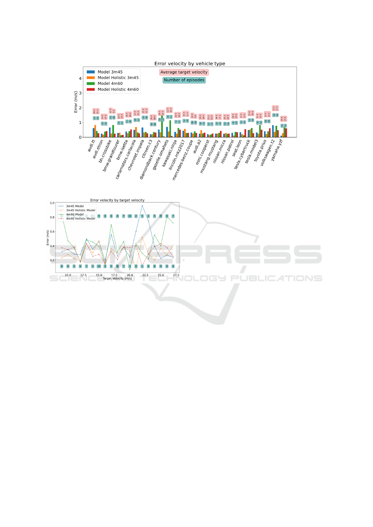
Figure 5: Error by Car Type. 3m 45º - 4m 60º.

Figure 6: Error by Target Speed. 3m 45º - 4m 60º.

this conﬁguration would be very small. Likewise, the

graph shows that the vehicles that show an improve-

ment in error are precisely those in which bicycles

have been simulated, vehicles whose behaviour was

more difﬁcult to predict by the individual model, and

therefore, with a greater possibility of error reduction.

Similarly, for the conﬁguration of the camera at a

height of 4m and a pitch of 60

◦

, there is a considerable

improvement in most cases, as this model had worse

results when using its own model. Moreover, this can

also be seen in Table 1, where we can see that when

testing the dataset with the model that only knows the

own images, the average error is 0.46m/s, while when

using the holistic model, this error has been reduced

to 0.33m/s.

On the other hand, in Figs. 5 and 6, it can also

be seen that while the 3m-45º dataset shows little im-

provement when using the holistic model, the 4m-

60º dataset does improve the error considerably, es-

pecially at high speeds.

In Figs. 7 and 8 the same behaviour can be ob-

served again. The holistic model improves in almost

all cases the individual model, and this can be ex-

plained in the same way as in the previous case, since

for both conﬁgurations of 4m 45º and 4m 60º they

record a lane stretch of approximately 9m and 5m re-

spectively, which is far from the minimum error zone.

Finally, recordings were made in a real environ-

ment at speeds of 30km/h, 50km/s and 70 km/h, us-

ing as ground truth the cruise control of a personal

vehicle and a LiDAR system positioned perpendicu-

lar to the plane of the lane. Using the holistic model

trained in simulation, individual errors were obtained

for each of the speeds of 4.12 m/s, 1.48 m/s and 0.93

m/s respectively.

These results can be considered satisfactory be-

cause it is a ﬁrst preliminary test, and the recordings

still have errors to correct, such as shutter and frame

rate, to match the images captured in simulation.

An example of a vehicle driving at 70km/h is

shown in the Fig. 9, where one of the problems iden-

tiﬁed when testing the recording, such as blur, can

be observed. The images taken have a resolution of

1920x1208 and have been recorded at 20 fps. To carry

out these tests, the camera was placed on a road with

two lanes in each direction of travel, at a height of 3.5

metres and centred on the lane to be recorded. At the

time of recording, the day was cloudy with no rain.

5 CONCLUSIONS AND FUTURE

WORKS

We can prove that a holistic model, which is trained

with a wide set of camera positions, can work for all

Towards View-invariant Vehicle Speed Detection from Driving Simulator Images

193

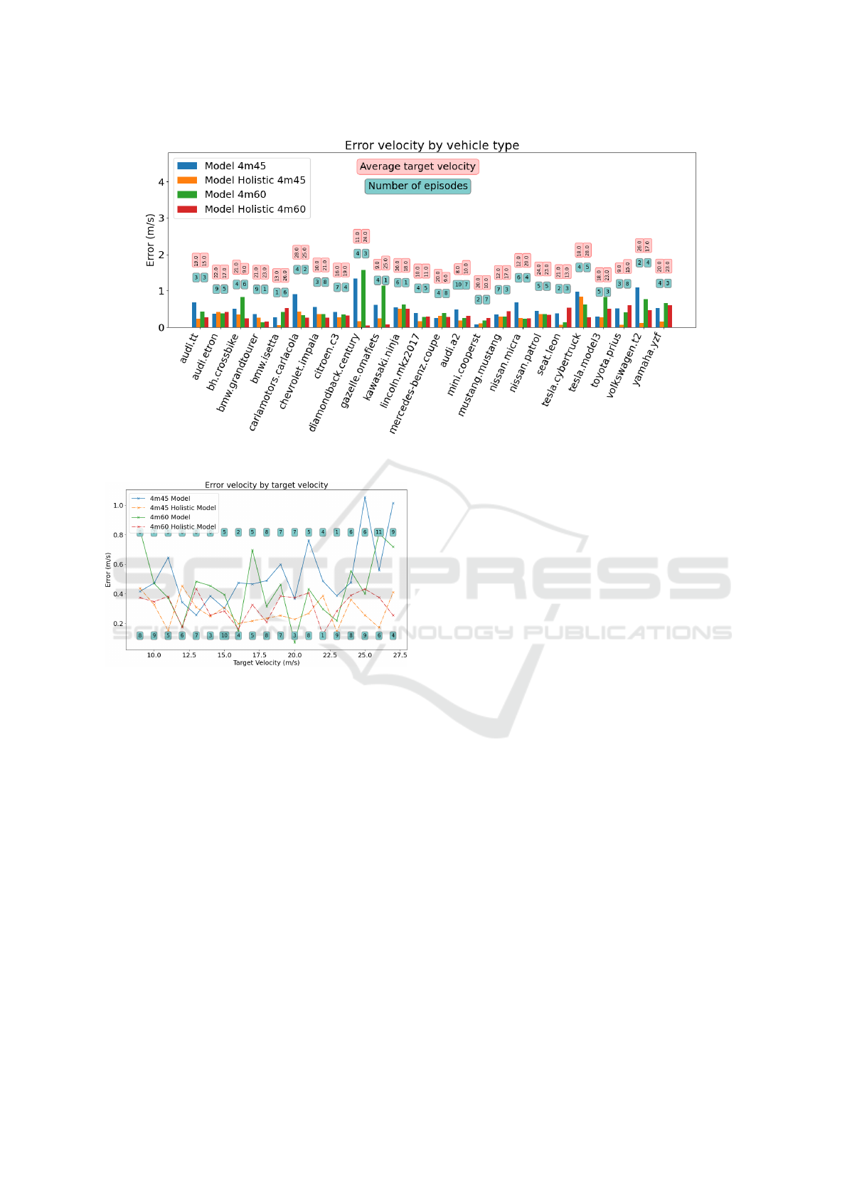
Figure 7: Error by Car Type. 4m 45º - 4m 60º.

Figure 8: Error by Target Speed. 4m 45º - 4m 60º.

of them, without the need to train a speciﬁc model for

each of the positions. Moreover, as has been shown

with real environment recordings, this model, which

has never seen this kind of images before, is able to

perform correctly.

These results indicate that it is possible to train a

model with an even larger set of camera positions, and

use it as a generic model for new and unknown posi-

tions for the network, obtaining sufﬁciently accurate

results.

The results obtained indicate that, if a model were

trained with a sufﬁciently large dataset, it could be ca-

pable of detecting the speed at which a vehicle is trav-

elling with greater accuracy than current radar-type

systems. Furthermore, it has also been shown that this

is also valid for other types of vehicles such as motor-

bikes, since a considerable improvement in error has

been seen in this type of vehicle with respect to the re-

sults obtained using only individual models. Finally,

a global model for any camera position would avoid

the work of having to train an individual model every

time a new system is placed in the real environment.

As future work, the plan is to take recordings of

longer duration, and in real trafﬁc situations in an ur-

ban environment, as well as to extend the simulation

training set, with new camera positions and different

trafﬁc directions, and to test it with different datasets

in which there are recordings in real environment in

different locations. In addition, the system can be

tested on a multi-lane road, trying to detect the speed

of vehicles in each lane individually, using computer

vision techniques.After this, we could try to imple-

ment a real time system on roads, obtaining data such

as the system’s computation speed, and also, being

able to be compared with other types of radars, whose

errors in the national territory, according to the atuori-

ties, oscillates between 5 and 7 km/h for speeds below

100km/h.

ACKNOWLEDGEMENTS

This work has been funded by research grant

SBPLY/19/180501/000093 (Community Region of

Castilla la Mancha), and partially funded by research

grants S2018/EMT-4362 SEGVAUTO 4.0-CM (Com-

munity Region of Madrid) and PID2020-114924RB-

I00 (Spanish Ministry Science Innovation)

KDIR 2022 - 14th International Conference on Knowledge Discovery and Information Retrieval

194

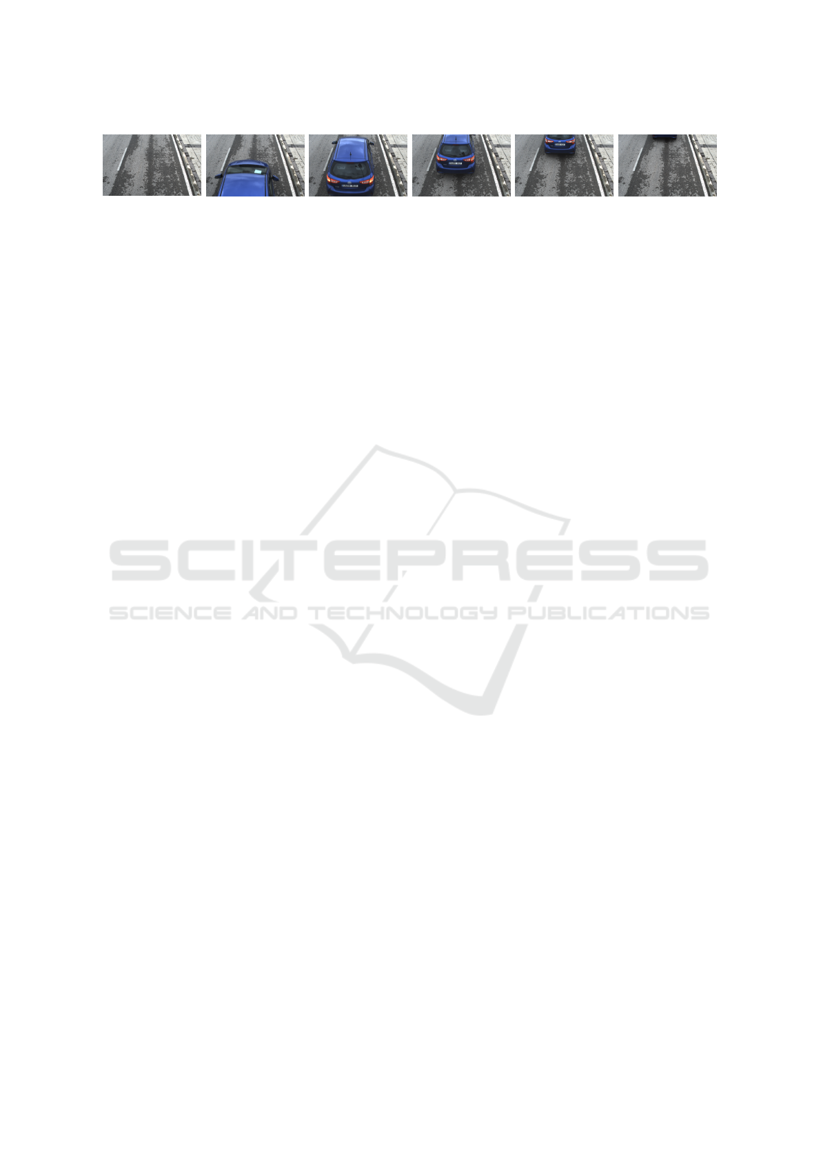
Figure 9: Real environment test. Sequence with a vehicle at 70km/h.

REFERENCES

Barros, J. and Oliveira, L. (2021). Deep speed estimation

from synthetic and monocular data. In 2021 IEEE In-

telligent Vehicles Symposium (IV), pages 668–673.

Biparva, M., Llorca, D. F., Izquierdo, R., and Tsotsos,

J. K. (2022). Video action recognition for lane-change

classiﬁcation and prediction of surrounding vehicles.

IEEE Transactions on Intelligent Vehicles.

Dong, H., Wen, M., and Yang, Z. (2019). Vehicle speed

estimation based on 3d convnets and non-local blocks.

Future Internet, 11.

Dosovitskiy, A., Ros, G., Codevilla, F., Lopez, A., and

Koltun, V. (2017). CARLA: An open urban driving

simulator. In Proceedings of the 1st Annual Confer-

ence on Robot Learning, pages 1–16.

Elvik, R. (2011). Developing an accident modiﬁcation func-

tion for speed enforcement. Safety Science, 49:920–

925.

ERSO, EC (2018). Speed enforcement 2018. European

Road Safety Observatory.

Fern

andez-Llorca, D., Hern

andez-Mart

ınez, A., and

Garc

ıa-Daza, I. (2021). Vision-based vehicle speed

estimation: A survey. IET Intelligent Transport Sys-

tems, 15(8):987–1005.

Lee, J., Roh, S., Shin, J., and et al. (2019). Image-based

learning to measure the space mean speed on a stretch

of road without the need to tag images with labels.

Sensors, 19.

Llorca, D. F., Salinas, C., Jim

enez, M., Parra, I., Morcillo,

A. G., Izquierdo, R., Lorenzo, J., and Sotelo, M. A.

(2016). Two-camera based accurate vehicle speed

measurement using average speed at a ﬁxed point.

In 2016 IEEE 19th International Conference on In-

telligent Transportation Systems (ITSC), pages 2533–

2538.

Luvizon, D. C., Nassu, B. T., and Minetto, R. (2017). A

video-based system for vehicle speed measurement in

urban roadways. IEEE Transactions on Intelligent

Transportation Systems, 18:1393–1404.

Madhan, E. S., Neelakandan, S., and Annamalai, R. (2020).

A novel approach for vehicle type classiﬁcation and

speed prediction using deep learning. Journal Comp.

Theor. Nano., 17:2237–2242.

Martinez, A. H., D

ıaz, J. L., Daza, I. G., and Llorca, D. F.

(2021). Data-driven vehicle speed detection from syn-

thetic driving simulator images. In 2021 IEEE Inter-

national Intelligent Transportation Systems Confer-

ence (ITSC), pages 2617–2622.

Parimi, A. and Jiang, Z. (2021). Dynamic speed estima-

tion of moving objects from camera data. In NAE-

CON 2021 - IEEE National Aerospace and Electron-

ics Conference, pages 307–316.

Revaud, J. and Humenberger, M. (2021). Robust automatic

monocular vehicle speed estimation for trafﬁc surveil-

lance. In 2021 IEEE/CVF International Conference

on Computer Vision (ICCV), pages 4531–4541.

Rodr

ıguez-Rangel, H., Morales-Rosales, L. A., Imperial-

Rojo, R., Roman-Garay, M. A., Peralta-Pe

nuri,

G. E., and Lobato-B

aez, M. (2022). Analysis of statis-

tical and artiﬁcial intelligence algorithms for real-time

speed estimation based on vehicle detection with yolo.

Applied Sciences, 12(6).

Sochor, J., Jur

anek, R., and Herout, A. (2017). Trafﬁc

surveillance camera calibration by 3d model bound-

ing box alignment for accurate vehicle speed measure-

ment. Computer Vision and Image Understanding,

161:87–98.

Wilson, C., Willis, C., Hendrikz, J. K., and et al. (2010).

Speed cameras for the prevention of road trafﬁc in-

juries and deaths. Cochrane Database of Systematic

Reviews, 11.

Towards View-invariant Vehicle Speed Detection from Driving Simulator Images

195