Root Cause Classification of Temperature-related Failure Modes in a

Hot Strip Mill

Samuel Latham and Cinzia Giannetti

Faculty of Science and Engineering, Swansea University, Fabian Way, Swansea, Wales

Keywords: Root Cause Analysis, Machine Learning, Classification, Data Analytics, Knowledge Integration, Hot Strip

Mill, Steel Industry.

Abstract: Data is one of the most valuable assets a manufacturing company can possess. Historical data in particular

has much potential for use in automated data-driven decision-making which can result in more efficient and

sustainable processes. Although the technology and research behind data-driven systems for Root Cause

Analysis has developed vastly over decades, their use for real time automated detection of root causes within

steel manufacturing has been limited. Typically, root cause analysis still involves a lot of human interaction

both in the pre-processing and data analysis phases, which can lead to variability in results and cause delay

when devising corrective actions. In this paper, an application for automated Root Cause Analysis in an Hot

Strip Mill is proposed for the purpose of demonstrating the effectiveness of such an approach against a manual

approach. The proposed approach classifies temperature defects of steel strip Width Pull using a variety of

machine learning algorithms in conjunction with k-fold cross validation.

1 INTRODUCTION

Each year, millions of tonnes of steel are rolled by

steel companies across the globe. While steel-making

plants strive to produce high quality steel strip and

limited waste, various defects still occur on a regular

basis and thousands of these are recorded by

operators each year. Width-related defects account

for a large portion of these.

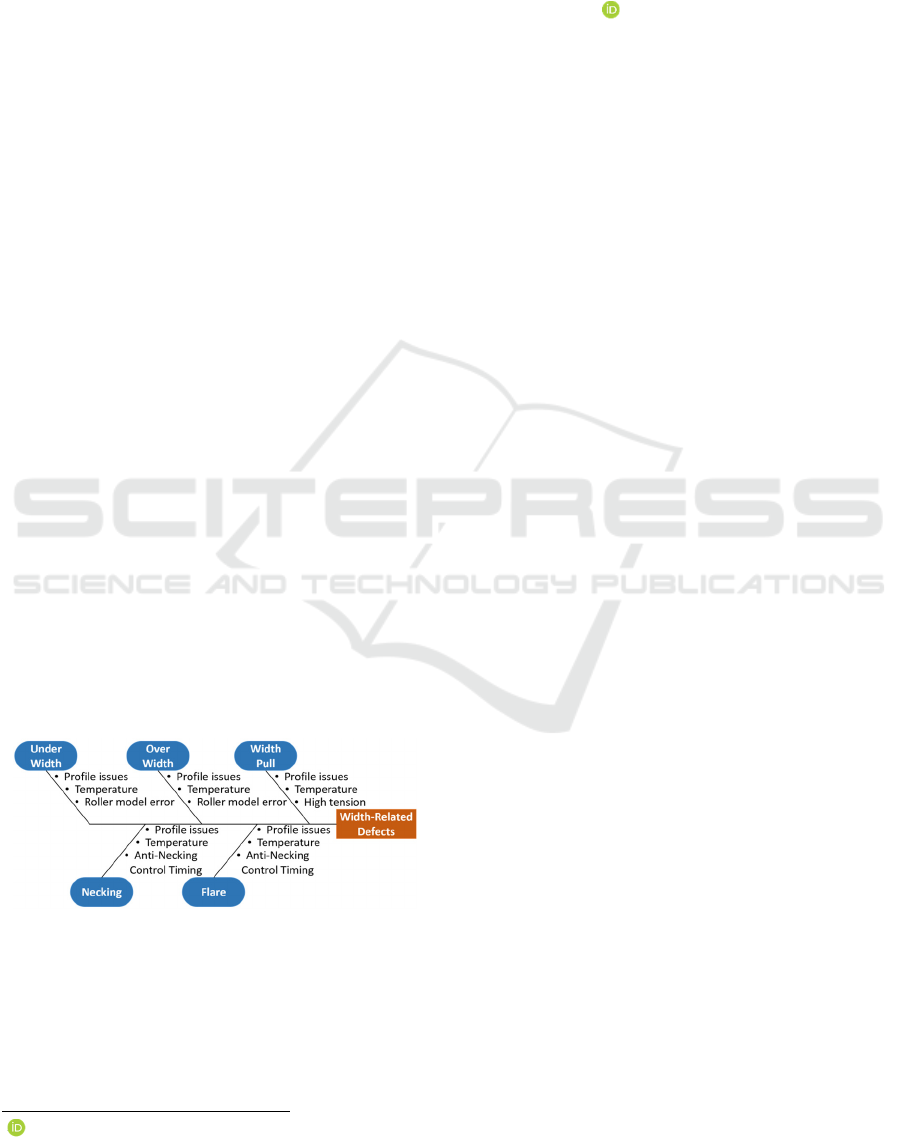
Figure 1: A fishbone diagram showing the causes of Width

Pull throughout an HSM.

There are several width-related defects, each with

a number of failure modes with potential origins from

various Hot Strip Mill (HSM) sub-processes,

including bar specification issues, temperature

fluctuations, and erratic tension control.

https://orcid.org/0000-0003-0339-5872

The current procedures used to determine the

causes of width-related defects, however, are mostly

manual and require human interaction before the

issue can be resolved, sometimes even including

simple true or false condition checks. This creates an

inconsistent timescale in which defects may go

unrecognised and successive products are therefore

negatively affected. These problems can occur not

only when defective behaviour is identified at a later

time, but also if defective behaviour is missed and

therefore goes unrecorded. Although human error is

thought to be the main concern associated with

manual processes, fast-paced and critical decision-

making and resource allocation are also primary

concerns (Janssen et al., 2019; Sheridan &

Parasuraman, 2000).

In recent decades, root cause analysis (RCA)

methodologies have adopted more up-to-date and

relevant technologies including automation and

machine learning (Mahto & Kumar, 2008).

Automation has proven to be a powerful approach in

manufacturing operations and RCA, dramatically

reducing the time between the occurrence of physical

events and digital analysis and visualisation

Oliveira et al., 2022), usually without the need for

Latham, S. and Giannetti, C.

Root Cause Classiﬁcation of Temperature-related Failure Modes in a Hot Strip Mill.

DOI: 10.5220/0011380300003329

In Proceedings of the 3rd International Conference on Innovative Intelligent Industrial Production and Logistics (IN4PL 2022), pages 36-45

ISBN: 978-989-758-612-5; ISSN: 2184-9285

human interaction. Machine learning also enables

RCA systems to learn patterns in data which can be

too ambiguous for a human to perceive and provides

the ability to re-train a system to adapt to new or

unforeseen behaviour (Wiering & van Otterlo, 2012;

Wuest et al., 2016). Within the steel rolling industry,

RCA, particularly with machine learning, is not yet

mainstream outside of its use in applications for

surface defect detection and roller model

optimisation. Currently, such applications have also

not been embedded into a larger RCA system

spanning multiple sub-processes in an HSM, which is

a future aim of this study.

By increasing the scope of machine learning

applications in an HSM setting, it is possible to create

a broad set of RCA tools for the identification of

failure modes which can be used to improve the

current process and reduce workload on team

members, allowing them to focus on other more

meaningful tasks. In the future, it would also be

beneficial to combine these tools into a broad system

to identify both the cause and origin of a defect

throughout a number of HSM sub-processes. This

would provide quick access and a simple but detailed

overview of the process with regards to process

performance and RCA.

In this paper, a proposition is made for an

automated RCA application which utilises machine

learning to classify the root cause of Width Pull in an

HSM. This aims to show that there is potential for a

series of this type of application to be created in a

steel industry setting and, in future, compiled into a

final system which can broadly monitor the HSM

process. The resulting application aims to save time

and boost productivity of both the HSM process and

analysts and reduce the overall number of defects that

occur in the future. In section 2, an insight into the

current issues and analysis procedures used in

existing HSMs is highlighted and a deeper

understanding into the background of RCA systems

and machine learning both in general and in the steel

industry is provided. The data pre-processing steps

taken and the methodology used to carry out

classification experiments are then outlined in section

3. The results of these experiments are then evaluated

against a manual approach to the described problem

in the penultimate section before concluding on the

proposed approach’s performance, the optimal

machine learning model, and how it might be

improved in the final section. Future work aims to

discuss the need and integration of such an

application in a broader RCA system spanning the

entire HSM process. This will be in conjunction with

a previous work in which an RCA application was

created for failure mode classification in an HSM

(Latham & Giannetti, 2021).

2 BACKGROUND

2.1 Root Cause Analysis in

Manufacturing and the Steel

Industry

2.1.1 Early Stages of Root Cause Analysis

Having only been around since the 1950s and only

becoming mainstream after the creation of Lean 6

Sigma in the 1980s, RCA has played a major part in

the push towards a better understanding of faults that

occur in manufacturing processes (Arnheiter &

Greenland, 2008; Ohno & Bodek, 1998). The aim of

RCA was originally to identify the cause of a known

issue so that an appropriate solution can then be

determined. However, the methodologies used to

achieve this goal has evolved over the years

(Arnheiter & Greenland, 2008) to make this process

more streamline and beneficial. Some examples

include the inclusion of expert knowledge, prescribed

solutions and, more recently, automation (Diez-

Olivan et al., 2019; Giannetti et al., 2015).

The first major example of a practical RCA

approach was the use of the 5 Whys methodology,

created in the 1930s by Toyota engineers

(Serrat,

2017), but becoming popular later in the century as

part of the Lean 6 Sigma framework . While Lean 6

Sigma is used to improve general business efficiency,

its techniques are often applied in the manufacturing

industry (Sreedharan & Raju, 2016). The 5 Whys

approach encourages further investigation into why

faults occur (Serrat, 2017), which, as mentioned, is

the main aim of RCA. The next major step in

developing RCA was to further include expert

knowledge such that analysts could make a guided

diagnosis of the issue (Sarkar, Mukhopadhyay, &

Ghosh, 2013). These expert systems eventually

included further knowledge such that a prescribed

solution could be given depending on the diagnosis

and inputs (Cao et al., 2022; Kalantri & Chandrawat,

2013). These were the first major steps towards

introducing artificial intelligence into RCA

methodologies.

2.1.2 Root Cause Analysis and Machine

Learning

Over the last few decades, the amount of data

collected in manufacturing processes has been

Root Cause Classiﬁcation of Temperature-related Failure Modes in a Hot Strip Mill

increasing at such a rate that it is becoming an

increasingly important challenge to make use of this

data in an efficient manner (Yaqoob et al., 2016).

However, the infrastructures in which such vast

amounts of data are stored are often unorganised and

require a number of processing steps (Madden, 2012)

before data is transformed into a suitable standard for

analysis. The inclusion of artificial intelligence has

propelled the development of RCA tools and

methodologies such that it is now possible to quickly

and efficiently process large amounts of information.

There are many examples which demonstrate such

tools which include the use of neural networks,

regression models, and other more traditional analysis

models such as control charts for automated RCA in

a variety of industries

(Oliveira et al., 2022; Giannetti

et al., 2014a, 2014b). However, some argue that

further development is still required to maximise its

potential (Zhang et al., 2020).

In the last several decades, machine learning has

become a very popular tool for quick and automated

analysis and feedback in manufacturing processes

(Cinar et al., 2020; Dogan & Birant, 2021; Essien &

Giannetti, 2019; Giannetti & Essien, 2022). The

premise of machine learning is to learn patterns from

the features of a given set of historical data and use

this information to create a model that can identify

these patterns in new, unseen data. This approach

attempts to automate manual RCA operations and

provide quick, if not immediate, feedback

(Steenwinckel, 2018).

There are many applications of RCA which utilise

machine learning in the manufacturing industry

(Weichert et al., 2019), and many unique approaches

have been taken to develop them. One such example

is the use of machine learning-based anomaly

detection methods, including K-Nearest Neighbour

(KNN) and Local Outlier Factor (LOF), to detect

failure modes in assembly equipment (Abdelrahman

& Keikhosrokiani, 2020). Another application

includes the use of machine learning, specifically

neural networks, for quality monitoring in an

injection moulding process (Nam, Van Tung, & Yee,

2021). One more example is the use of supervised

methods such as K-Means Clustering and decision

trees for the detection of root causes of defects in

semiconductors (Tan et al., 2021). It is worth noting

that some approaches argue that a knowledge-based

approach can sometimes be more suitable than

machine learning depending upon the scenario

(Martinez-Gil et al., 2022; Roshan et al., 2014). It is

clear that some solutions are chosen to cater to the use

case addressed by the application but have the

common goal of using information from a process to

provide useful feedback for the purpose of improving

a process (Weichert et al., 2019).

2.1.3 Root Cause Analysis in the Steel

Rolling Industry

Within the steel rolling industry machine learning

and, especially, RCA is not yet mainstream and has

only seen analytics for RCA used on a niche scale.

While there has been much development for existing

applications of machine learning, areas of focus in

research are largely limited to surface defect detection

(Huang, Wu, & Xie, 2021) and roller model

optimisation (Li, Luan, & Wu, 2020). While it may

be difficult to introduce new technologies into an

operation of such a scale, machine learning has

untapped potential with regards to RCA in the steel

industry as it would enhance the automation of such

analyses. Time and resources spent on conducting

this process manually would therefore be saved and

workers who would normally be tasked with this

could devote more time to other workloads or more

complex projects in which human interaction is a

necessity.

2.2 Width Pull and Current HSM

Procedures

2.2.1 Width Pull in the HSM

When Width Pull occurs, the head end of a steel bar

either elongates or becomes under width specification

as a result of sudden tension in the strip (Khramshinet

al., 2015; Radionov et al., 2020). This defect can

occur for an array of reasons, including wrong bar

specifications, high or low temperatures, and erratic

tension.

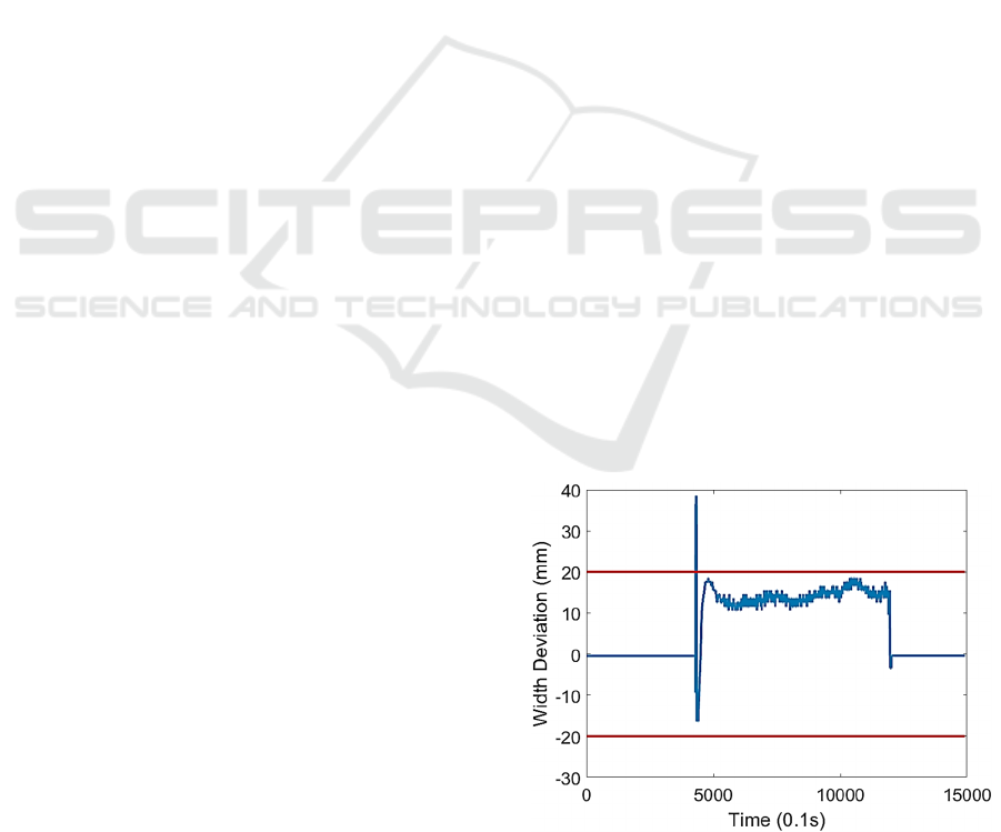
Figure 2: A graph showing the width deviation of a strip

with Width Pull.

IN4PL 2022 - 3rd International Conference on Innovative Intelligent Industrial Production and Logistics

Currently, when Width Pull occurs in the HSM,

the root cause is determined via a manual analysis of

the defective sample. There are many causes of Width

Pull and, although there is a workflow in place to

determine basic causes, the data examined to

determine other causes can be quite ambiguous

making them difficult to draw conclusions on.

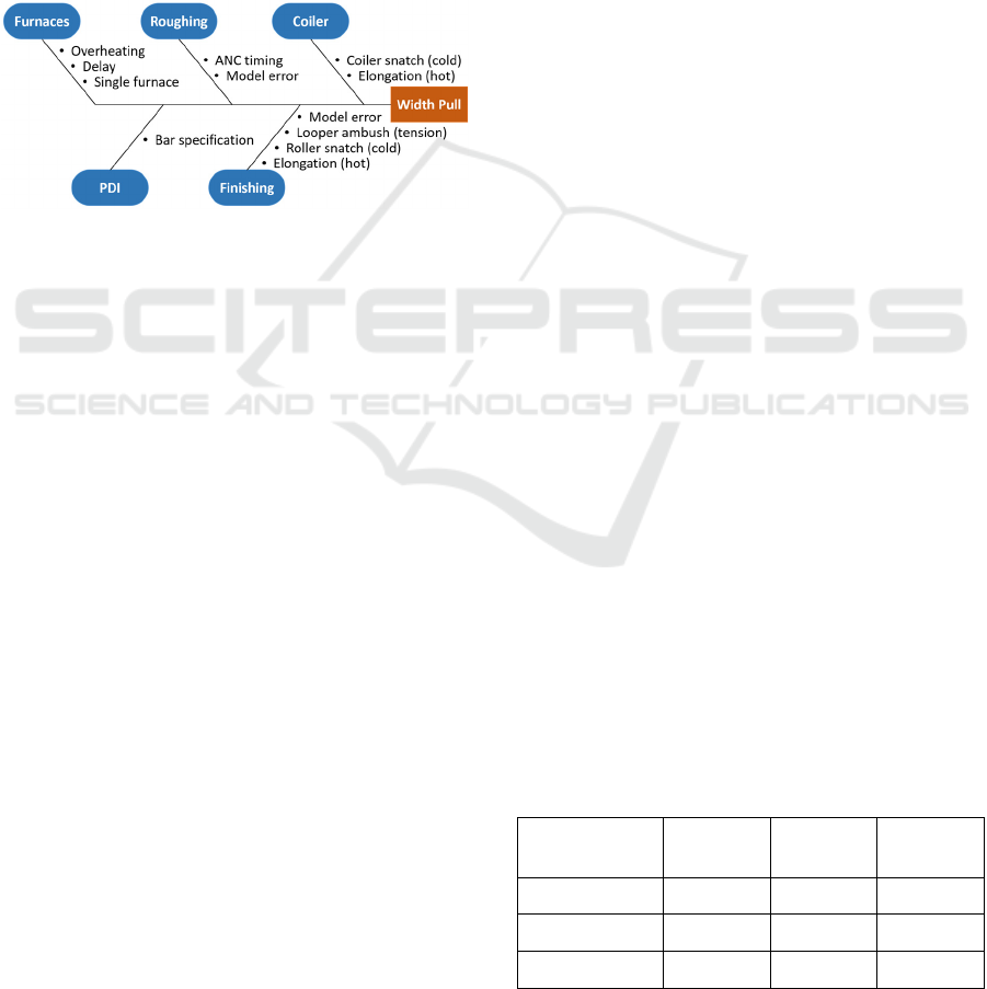
Although temperature-related causes normally

originate from the furnace (as shown in Figure 3), it

is important to note that the issue is originally

identified in a later part of the HSM process such as

Roughing or Finishing. Many failure modes of width-

related defects in the HSM process are temperature-

related (as shown in Figure 1).

Figure 3: A fishbone diagram showing the causes of Width

Pull throughout a HSM.

2.2.2 Current HSM Procedures

Width Pull, as well as other defects that occur in the

HSM, can have damaging effects both in the short-

term and long-term. Depending on the severity of the

under width caused by Width Pull or other defects, a

follow-up action is carried out. The first possible

action is a cutback in which the under width portion

of the strip is cut off. This results in a shorter strip

length and scrap which is melted for use in later strips,

requiring further processing which is both time-

consuming and unresourceful. Another action is to

make a concession in which the customer is offered

the defective strip at a negotiated lower price.

Although this action does not always require further

processing, potential profit is still lost. This however

does not mean that cutbacks do not occur before or

after concessions are made. In the worst-case

scenario, the strip is scrapped altogether. In the long-

term, all follow up actions require either further

resources and cost time and money, or result in

wasted material, ultimately producing business waste

(Sarkar, Mukhopadhyay, & Ghosh, 2013; Sreedharan

& Raju, 2016).

The effects of these defects can also be derived

not just from the defect itself but from the manual

analysis process that is currently used to determine

their root causes. Issues are often caught or resolved

long after immediate and, sometimes, lasting impacts

that are created by defective behaviour. For example,

some causes of Width Pull can affect a sequence of

strips if left unresolved (Khramshin et al., 2015). A

build-up of unresolved issues also suggests that the

information collected about root causes is analysed

too late to have a meaningful impact on the process,

resulting in a less productive system. Lastly, manual

analysis is time-consuming for analysts themselves. It

is a trivial task which, if automated, would enable

them to focus on more complex tasks and other

responsibilities, thus boosting their productivity.

3 METHODOLOGY

3.1 Problem Statement

In the following experiments, the potential of

machine learning for automating RCA in an HSM

setting is demonstrated by classifying temperature-

related failure modes of steel strips which have

suffered from Width Pull. This application is planned

to be part of a greater work which will combine such

applications and determine the failure mode and

origin of identified strips with Width Pull throughout

the HSM.

3.2 Dataset

The number of steel strips affected by low

temperature, or ‘undersoaking’, accounts for a larger

percentage of samples, overall making the dataset

used in this study unbalanced. At the time of data

collection, a total of 166 samples were available, 111

of which were undersoaked and 55 of which were

high temperature. Despite the imbalance, the

available dataset still had a limited number of

samples. It was therefore decided to use the whole

dataset for this experiment rather than reducing the

amount of undersoaked samples to account for

balance, which would limit the quality of training

during machine learning.

Table 1: A table showing the split of labelled data used in

this experiment.

Training

Dataset

Testing

Dataset

Total

(Label)

Undersoaked 78 33 111

High Temp 39 16 55

Total (Dataset) 117 49 166

Root Cause Classiﬁcation of Temperature-related Failure Modes in a Hot Strip Mill

Each sample is derived from two temperature

signals which are pre-processed and compared to

evaluate their representation of the root cause. This is

achieved through a series of transformations which

eliminate redundant data and account for differing

temperature ranges between different product

specification and comparing the range of values

between different product specifications and

comparing the range of values between the two

signals following these transformations. Statistical

features are then chosen to represent the samples

during the training stage of machine learning. These

features help the chosen machine learning algorithms

to distinguish between the behaviour of undersoaking

and high temperature.

3.3 Pre-processing and Labelling

In order to analyse the signal data both manually and

using machine learning, redundant data must first be

eliminated and, if it is not already, the remaining data

must be processed into a readable format. By cleaning

signal data like this, a more relevant perspective of

our data is shown, making data from different classes

more distinct during the feature extraction stage. The

first step is to eliminate irrelevant measurements in

the signal which occur when the bar is not present in

the Finishing Mill (as shown in Figure 4). A binary

Metal-In-Mill (MIM) signal displays whether or not

the bar is present in the mill. The second step is

completed by extracting the temperature signal

measurement where the MIM signal is activated (as

shown in Figure 5).

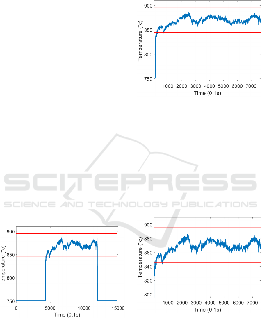
Figure 4: Temperature signal of an undersoaked strip before

pre-processing.

Figure 5: Temperature signal of an undersoaked strip where

MIM signal is activated.

The second step is to pad outlier measurements to

sensible values (as shown in Figure 6). Measurements

above a strip temperature’s upper tolerance plus 50°c

are set to this value. Alternatively, measurements

below a strip temperature’s lower tolerance minus

50°c are set to this value. Outlier values alone are not

enough to distinguish whether Width Pull is caused

by temperature. This is because these values may be

caused by erroneous sensor readings and, very

commonly, noise upon the strip’s entrance into the

Finishing Mill. Data representing this behaviour is

therefore eliminated from the beginning of the signal

to remove redundant values that may misrepresent

failure modes during training.

Figure 6: Temperature signal of an undersoaked strip after

outliers are removed.

The next step in narrowing down on this

information is to segment first 10% of the signal,

representing the head end of the strip (as shown in

Figure 7). This is because Finishing Mill Width Pull

IN4PL 2022 - 3rd International Conference on Innovative Intelligent Industrial Production and Logistics

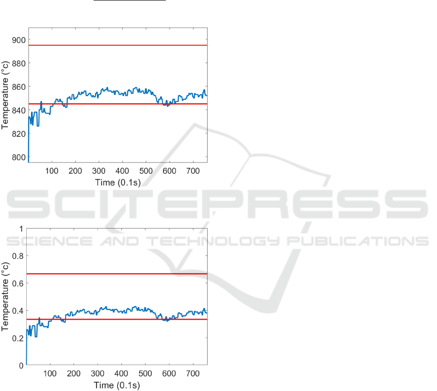
instances typically occur in the head end of the bar.

The final step maps each signal to a comparable scale

such that measurement ranges are mapped to the

sample values. A standard peak normalisation

formula (1) is used with the minimum and maximum

values of each signal to map all values of all signals

between 0 and 1 (as shown in Figure 8).

𝑃𝑒𝑎𝑘 𝑁𝑜𝑟𝑚. 

𝑥min



𝑥

max



𝑥  min



𝑥

(1)

Figure 7: Temperature signal representing the head end of

an undersoaked strip.

Figure 8: Temperature signal of an undersoaked strip after

peak normalisation.

Although basic labels exist to show simply

whether or not a steel strip sample is has Width Pull,

the data required for this application must be specific

to the root cause of the defect. Using a combination

of the existing manual analysis process, the extracted

data, and a series of plots displaying the now cleaned

signal data, the root causes of the extracted Width

Pull samples were manually labelled, creating further

labels used to train and test the final machine learning

algorithms.

3.4 Feature Selection

A collection of statistical features was extracted from

the pre-processed data for use in the chosen machine

learning algorithms. These include several quartile

values, mean, peak value, root mean square, and

standard deviation. Pearson’s Correlation Coefficient

was then used to determine which of these features

would be used during training. More specifically, the

averages of each feature after being applied to this

formula were used as a guide to eliminate features

which correlated too closely and would therefore

become redundant or counterproductive during

training (Schober, Boer, & Schwarte, 2018). The

result of this methodology is a feature set which is

combined with the labels to create a final dataset

which can be used to train and test the machine

learning model appropriately.

3.5 Machine Learning Algorithms

A variety of classic machine learning algorithms has

been selected for training and testing in this

experiment. This subsection briefly describes each

model and their parameters.

3.5.1 Trees

A classification tree is a linear graph in which each

node is assigned a value based on training features.

These values are used as a foundation for decision-

making when classifying new samples.

3.5.2 Naïve Bayes

Naïve Bayes also uses probabilities based on training

features to determine classification labels. However,

the Naïve Bayes algorithm bases these probabilities

on the frequency of each value, meaning that more

prominent features are dominant in classification.

3.5.3 K-Nearest Neighbour

The KNN algorithm creates a dimensional space in

which samples are plotted based on the values of their

features. New samples are plotted in this space and

compared to a chosen number, k, of neighbours. The

class of a new sample is chosen based on the class of

the majority of its k neighbours. It should be noted

that the numbers k in KNN and k-fold cross validation

are unrelated.

Root Cause Classiﬁcation of Temperature-related Failure Modes in a Hot Strip Mill

3.5.4 Support Vector Machines

A Support Vector Machine (SVM) also plots feature

values into a dimensional space, although rather than

comparing new samples to a distribution, this

algorithm attempts to create a new, separating

hyperplane. New samples are classified based on their

position relative to this hyperplane.

3.5.5 Artificial Neural Networks

Artificial Neural Networks (ANNs) are made up of

neurons which are combined to form a number of

layers. Each neuron has a weight which is updated

during training based on the inputted features. An

ANN’s width and depth is determined by the number

of neurons and layers it contains.

3.5.6 Ensembles

An ensemble combines the result of more than one

machine learning algorithm. The ensembles used in

this experiment combines several tree algorithms.

3.6 K-fold Cross Validation

K-fold cross validation is used to estimate the

generalisation error of a machine learning model. In

this experiment, k = 5 has been chosen such that each

machine learning algorithm is run five times using

80% of the training dataset. For each of the five runs,

20% is not used during training.

4 RESULTS

4.1 Full Training Dataset

A total of 13 machine learning algorithms were used

in the training stage of this experiment. Accuracy,

precision, recall, and F1 score metrics are used to

evaluate the performance of each model. Accuracy

simply calculates the overall percentage of correctly

labelled samples. Precision describes the percentage

of samples which are labelled as a given class that

truly belong to this class while recall describes the

percentage of samples which belong to this class that

are classified correctly. Although accuracy is still an

informative metric, F1 score is derived from precision

and recall, and evaluates the performance of

classification models more reliably. In the following

results, F1 score is represented as a percentage for

consistency among metrics.

Table 2: Performance of each machine learning algorithm

when trained on the full training dataset.

Algorithm

Accuracy

(%)

Precision

(%)

Recall

(%)

Score

(%)

Coarse

Gaussian

SVM

93.88 88.24 93.75 90.91

Coarse

Tree

95.92 93.75 93.75 93.75

Fine

Gaussian

SVM

81.63 81.82 56.25 66.67

Fine KNN 87.76 85.71 75 80

Fine Tree 95.92 93.75 93.75 93.75

Gaussian

Naïve

Bayes

93.88 84.21 1 91.43

Kernel

Naïve

Bayes

95.92 88.89 1 94.12

Linear

SVM

91.84 87.5 87.5 87.5

Narrow

ANN

93.88 93.33 87.5 90.32

Opt.

Ensemble

91.84 87.5 87.5 87.5

Opt. ANN 93.88 93.33 87.5 90.32

Quadratic

SVM

91.84 87.5 87.5 87.5

Wide ANN 89.8 86.67 81.25 83.97

From the results shown in Table 2, it can be seen

that a majority of the trained models can be used

appropriately for the classification task. However,

only a handful show consistent scores between the

performance metrics. In particular, the Coarse and

Fine Tree models have been shown to perform best

with accuracies and F1 scores of above 93%. These

models are generally quick to train and thus easier to

retrain when more data becomes available. Although

the Kernel Naïve Bayes model provides a better

accuracy, recall, and F1 score, its precision falls

behind the two Tree models, suggesting it does not

perform as well when labelling a particular class.

4.2 K-fold Cross Validation

After 5-fold cross validation, the models show

slightly decreased but similar performance to the

previous test results (as shown in Table 3). This

means that although each algorithm was given less

information during training, the models were still able

IN4PL 2022 - 3rd International Conference on Innovative Intelligent Industrial Production and Logistics

to generalise data relatively well, resulting in stable

training and thus reliable and consistent models.

Table 3: Performance of each machine learning algorithm

in 5-fold cross validation.

Algorithm

Accuracy

(%)

Precision

(%)

Recall

(%)

Score

(

)

Coarse

Gaussian

SVM

85.31 79.01 75 76.88

Coarse

Tree

88.37 83.8 80 81.73

Fine

Gaussian

SVM

87.89 82.78 79.58 81.06

Fine KNN 88.16 82.55 80.94 81.63

Fine Tree 88.82 83.76 81.75 82.62

Gaussian

Naïve

88.64 82.59 83.13 82.64

Kernel

Naïve

88.57 81.94 83.93 82.7

Linear

SVM

88.47 81.76 83.75 82.55

Narrow

ANN

88.57 82.55 83.19 82.54

Opt.

Ensemble

88.86 82.69 84 83.03

Opt. ANN 88.79 82.47 84.09 82.98

Quadratic

SVM

88.74 82.46 83.85 82.87

Wide ANN 88.73 82.72 83.46 82.78

While it is beneficial to determine whether a

machine learning model generalises well, as has been

shown in this experiment, the Tree-based models

would be likely to be selected for use in this

application based on their superior performance in the

full training experiment (as shown in Table 2). In this

particular cross validation experiment, the

Optimisable Ensemble performed marginally better

than other models, but would not be selected for use

in the final application based on its performance when

trained on the full dataset.

At the current time, the small dataset used in this

experiment is suitable for the application of

classifying temperature-related root causes of Width

Pull. However, using the best performing machine

learning algorithms in this experiment, it will be both

time and cost-efficient to retrain with more data at a

later date.

5 CONCLUSION

A digitised version of the current RCA system for

Width Pull in an existing HSM has been proposed and

has shown to perform acceptably for the given task. It

is capable of providing almost immediate results and

feedback, dramatically reducing the time between a

defect occurring and its root cause being identified.

There would be several benefits of adopting this

application into an HSM setting. Time would be

saved on performing unnecessary analyses, reserving

efforts for productivity elsewhere. This application

also showcases the potential of combining data

sources with the aim of repurposing data to create

new tools and maximise the value of data resources.

This application is a step towards further automation

and digitisation of basic HSM analyses and shows

this approach has the potential to reduce workload on

analysts such that human interaction can be directed

towards more complex issues in the HSM. In future

work, there may also be potential in applying this

methodology to other steel strip manufacturing

processes, such as casting and cold rolling, and

linking the analyses of root causes between these

processes.

ACKNOWLEDGEMENTS

The authors would like to acknowledge the M2A

funding from the European Social Fund via the Welsh

Government (c80816) and Tata Steel Europe that has

made this research possible. Prof. Giannetti would

like to acknowledge the support of the UK

Engineering and Physical Sciences Research Council

(EP/V061798/1). All authors would like to

acknowledge the support of the IMPACT and

AccelerateAI projects, part-funded by the European

Regional Development Fund (ERDF) via the Welsh

Government.

REFERENCES

Abdelrahman, O., & Keikhosrokiani, P. (2020). Assembly

Line Anomaly Detection and Root Cause Analysis

Using Machine Learning. IEEE Access, 8(1), 189661–

189672.

Arnheiter, E. D., & Greenland, J. E. (2008). Looking for

root cause: a comparative analysis. In The TQM

Journal, 20(1), 18–30.

Cao, Q., Zanni-Merk, C., Samet, A., Reich, C., de Beuvron,

F., Beckmann, A., & Giannetti, C. (2022). KSPMI: A

Knowledge-based System for Predictive Maintenance

Root Cause Classiﬁcation of Temperature-related Failure Modes in a Hot Strip Mill

in Industry 4.0. Robotics and Computer-Integrated

Manufacturing, 74(11), 1–15.

Cinar, Z., Nuhu, A., Zeeshan, Q., Korhan, O., Asmael, M.,

& Safaei, B. (2020). Machine Learning in Predictive

Maintenance towards Sustainable Smart Manufacturing

in Industry 4.0. Sustainability, 12(19), 1–36.

Diez-Olivan, A., Del Ser, J., Galar, D., & Sierra, B. (2019).

Data fusion and machine learning for industrial

prognosis: Trends and perspectives towards Industry

4.0. Information Fusion, 50(1), 92–111.

Dogan, A., & Birant, D. (2021). Machine learning and data

mining in manufacturing. Expert Systems with

Applications, 166(2), 11–19.

Essien, A., & Giannetti, C. (2019). A Deep Learning

Framework for Univariate Time Series Prediction

Using Convolutional LSTM Stacked Autoencoders.

IEEE International Symposium on Innovations in

Intelligent Systems and Applications, 1–6.

Giannetti, C., & Essien, A. (2022). Towards Scalable and

Reusable Predictive Models for Cyber Twins in

Manufacturing Systems. Journal of Intelligent

Manufacturing, 33(2), 441–455.

Giannetti, C., Ransing, M. R., Ransing, R. S., Bould, D. C.,

Gethin, D. T., & Sienz, J. (2015). Organisational

Knowledge Management for Defect Reduction and

Sustainable Development in Foundries. International

Journal of Knowledge and Systems Science, 6(3), 18–

37.

Giannetti, C., Ransing, M., Ransing, R., Bould, D. C.,

Gethin, D. T., & Sienz, J. (2014a). Product specific

process knowledge discovery using co-linearity index

and penalty functions to support process FMEA in the

steel industry. CIE 2014 - 44th International

Conference on Computers and Industrial Engineering

and IMSS 2014 - 9th International Symposium on

Intelligent Manufacturing and Service Systems, Joint

International Symposium on "The Social Impacts of

Developments in Information. 1–15.

Giannetti, C., Ransing, R., Ransing, M. R., Bould, D. C.,

Gethin, D. T., & Sienz, J. (2014b). A novel variable

selection approach based on co-linearity index to

discover optimal process settings by analysing mixed

data. Computers & Industrial Engineering, 72(1), 217–

229.

Huang, Z., Wu, J., & Xie, F. (2021). Automatic recognition

of surface defects for hot-rolled steel strip based on

deep attention residual convolutional neural network.

Materials Letters, 293(1), 3049–3055.

Janssen, C. P., Donker, S. F., Brumby, D. P., & Kun, A. L.

(2019). History and future of human-automation

interaction. International Journal of Human-Computer

Studies, 131(1), 99–107.

Kalantri, R., & Chandrawat, S. (2013). Root Cause

Assessment for a Manufacturing Industry: A Case

Study. Journal of Engineering Science and Technology

Review, 6(1), 62–67.

Khramshin, V. R., Evdokimov, S. A., Yu, A. I., Shubin, A.

G., & Karandaev, A. S. (2015). Algorithm of no-pull

control in the continuous mill train. 2015 International

Siberian Conference on Control and Communications

(SIBCON). 1–5.

Latham, S., Giannetti, C. (2021). Pre-Trained CNN for

Classification of Time Series Images of Anti-Necking

Control in a Hot Strip Mill. The 9

IIAE International

Conference on Industrial Engineering 2021

(ICIAE2021). 77–84.

Li, X., Luan, F., & Wu, Y. (2020). A Comparative

Assessment of Six Machine Learning Models for

Prediction of Bending Force in Hot Strip Rolling

Process. Metals, 10(5), 1–16.

Madden, S. (2012). From Databases to Big Data. In IEEE

Internet Computing, 16(3), 4–6.

Mahto, D., & Kumar, A. (2008). Application of root cause

analysis in improvement of product quality and

productivity. Journal of Industrial Engineering and

Management, 1(2), 16–53.

Martinez-Gil, J., Buchgeher, G., Gabauer, D.,

Freudenthaler, B., Filipiak, D., & Fensel, A. (2022).

Root Cause Analysis in the Industrial Domain using

Knowledge Graphs: A Case Study on Power

Transformers. Procedia Computer Science, 200(3),

944–953.

Murugaiah, U., Benjamin, S. J., Marathamuthu, M. S., &

Muthaiyah, S. (2010). Scrap loss reduction using the 5-

whys analysis. International Journal of Quality &

Reliability Management, 27(5), 527–540.

Nam, D. N. C., Van Tung, T., & Yee, E. Y. K. (2021).

Quality monitoring for injection moulding process

using a semi-supervised learning approach. IECON

2021 – 47th Annual Conference of the IEEE Industrial

Electronics Society. 1–6.

Ohno, T., & Bodek, N. (1988). Toyota Production System:

Beyond Large-Scale Production (1st Edition).

Productivity Press. 136–142.

Oliveira, E., Miguéis, V. L., & Borges, J. (2022). Automatic

root cause analysis in manufacturing: an overview &

conceptualization. Journal of Intelligent

Manufacturing, 33(5), 1–18.

Radionov, A. A., Gasiyarov, V. R., Karandaev, A. S.,

Usatiy, D. Y., & Khramshin, V. R. (2020). Dynamic

Load Limitation in Electromechanical Systems of the

Rolling Mill Stand during Biting. 2020 IEEE 11

International Conference on Mechanical and

Intelligent Manufacturing Technologies (ICMIMT).

149–154.

Roshan, H., Giannetti, C., Ransing, M., & Ransing, R.

(2014). "If only my foundry knew what it knows…" : a

7Epsilon perspective on root cause analysis and

corrective action plans for ISO9001:2008. 71st World

Foundry Congress: Advanced Sustainable Foundry,

WFC 2014. 1–15.

Sarkar, A., Mukhopadhyay, A., & Ghosh, S. (2013). Root

cause analysis, Lean Six Sigma and test of hypothesis.

The TQM Journal, 25(2), 170–185.

Schober, P., Boer, C., & Schwarte, L. A. (2018).

Correlation coefficients: appropriate use and

interpretation. Anesthesia & Analgesia, 126(5), 1763–

1768.

IN4PL 2022 - 3rd International Conference on Innovative Intelligent Industrial Production and Logistics

Serrat, O. (2017). The Five Whys Technique. Knowledge

Solutions (1st Edition). Springer. 307–310.

Sheridan, T., & Parasuraman, R. (2000). Human Versus

Automation in Responding to Failures: An Expected

Value Analysis. Human Factors, 42(3), 403–407.

Sreedharan, V. R., & Raju, R. (2016). A systematic

literature review of Lean Six Sigma in different

industries. International Journal of Lean Six Sigma,

7(4), 430–466.

Steenwinckel, B. (2018). Adaptive anomaly detection and

root cause analysis by fusing semantics and machine

learning. European Semantic Web Conference. 272–

282.

Tan, D., Xu, X., Yu, K., Zhang, S., & Chen, T. (2021).

Multi-Feature Shuffle Algorithm for Root Cause

Detection in Semiconductor Manufacturing. 2021 IEEE

Intl Conf on Dependable, Autonomic and Secure

Computing, Intl Conf on Pervasive Intelligence and

Computing, Intl Conf on Cloud and Big Data

Computing, Intl Conf on Cyber Science and Technology

Congress (DASC/PiCom/CBDCom/CyberSciTech).

130–136.

Weichert, D., Link, P., Stoll, A., Rüping, S., Ihlenfeldt, S.,

& Wrobel, S. (2019). A review of machine learning for

the optimization of production processes. The

International Journal of Advanced Manufacturing

Technology, 104(9), 1889–1902.

Wiering, M., & van Otterlo, M. (2012). Reinforcement

Learning: State-of-the-Art (2012 Edition). Springer. 3–

32.

Wuest, T., Weimer, D., Irgens, C., & Thoben, K.-D. (2016).

Machine learning in manufacturing: Advantages,

challenges, and applications. Production &

Manufacturing Research, 4(1), 23–45.

Yaqoob, I., Hashem, I. A. T., Gani, A., Mokhtar, S.,

Ahmed, E., Anuar, N. B., & Vasilakos, A. V. (2016).

Big data: From beginning to future. International

Journal of Information Management, 36(6), 1231–

1247.

Zhang, J., Arinez, J., Chang, Q., Gao, R., & Xu, C. (2020).

Artificial Intelligence in Advanced Manufacturing:

Current Status and Future Outlook. Journal of

Manufacturing Science and Engineering, 142(1), 1–53.

Root Cause Classiﬁcation of Temperature-related Failure Modes in a Hot Strip Mill