
Making Hard(Er) Bechmark Test Functions
Dante Niewenhuis
1 a
and Daan van Den Berg
2 b
1
Master Artificial intelligence, Informatics Institute, University of Amsterdam, The Netherlands
2
Department of Computer Science, Vrije Universiteit Amsterdam, The Netherlands
Keywords:
Evolutionary Algorithms, Continuous Problems, Benchmarking, Instance Hardness.
Abstract:
This paper is an exploration into the hardness and evolvability of default benchmark test functions. Some very
well-known traditional two-dimensional continuous benchmark test functions are evolutionarily modified to
challenge the performance of the plant propagation algorithm (PPA), a crossoverless evolutionary method. For
each traditional benchmark function, only its scalar constant parameters are mutated, but the effect on PPA’s
performance is nonetheless enormous, both measured in objective deficiency and in the success rate. Thereby,
a traditional benchmark functions’ hardness can thereby indeed be evolutionarily increased, and an especially
interesting observation is that the evolutionary processes seem to follow one of three specific patterns: global
minimum narrowing, increase in ruggedness, or concave-to-convex inversion.
1 BENCHMARK TEST
FUNCTIONS
Sure there’s free lunch. Depth-first branch and bound
outperforms an exhaustive search on the entirety of
traveling salesman problem instances, when paid in
recursions. But when it comes to iterative (stochas-
tic) algorithms, which may or may not “have drawn
inspiration from optimization that occur in nature”,
Wolpert & Macready’s No Free Lunch Theorem
states that “the average performance of any pair of
algorithms across all possible problems is identical”
(Wolpert and Macready, 1997). This a very strong
result, and may even be somewhat disheartening to
those hoping to find a general-purpose optimization
algorithm (Brownlee et al., 2007).
So to what extent are Wolpert & Macready
(in)directly responsible for the popularity of bench-
marking practices in iterative optimization? Recently,
no less then 17 leading scientists coauthored a paper
on benchmarking evolutionary algorithms a few years
ago. “Benchmarking in Optimization: Best Practice
and Open Issues” is still actively under development
(currently in its third version) and shows that the sub-
ject’s debate is active (Bartz-Beielstein et al., 2020). It
affirms that the community’s focus from ‘finding the
best optimization algorithm’ in general has shifted to
a
https://orcid.org/0000-0002-9114-1364
b
https://orcid.org/0000-0001-5060-3342
‘finding the best optimization algorithm for a certain
problem (instance)’ (Rice, 1976)(Kerschke and Traut-
mann, 2019). This could be seen as a direct or indirect
partial consequence of the free lunch theorem.
Benchmark sets come in many various forms for
various problems, and appear to be selected on ba-
sis reputation mostly. One such example is Reinelt’s
TSPLIB, a benchmark set for the traveling salesman
problem (Reinelt, 1991). Not particularly suitable for
complexity tests, but valuable in their practicality, the
set contains 144 problem instances of Euclidean TSP,
mostly real-world maps, but also ‘real’ drilling plans.
Stemming from 1991, such an early benchmark set
has allowed many scientists to test their algorithms
on the same problem instances for quite some time.
Other examples include cutting and packing problem
instances (Iori et al., 2021a; Iori et al., 2021b; Iori
et al., 2021c)(Braam and van den Berg, 2022), the job
shop scheduling problem (Weise et al., 2021) pseudo-
Boolean optimization (Doerr et al., 2020) and the W-
model problem (Weise and Wu, 2018a)(Weise and
Wu, 2018b).
These examples are all benchmark sets for ‘dis-
crete’ optimization problems, usually meaning the
number of solutions is finite, even though the objec-
tive function can still be continuous. Contrarily, in
the class of continuous optimization problems, the
variables are instantiated from a numeric range (such
as −4 ≤ x
1
, x
2
≤ 5), hence there is an infinite num-
ber of solutions. Although not strictly required, con-
Niewenhuis, D. and van Den Berg, D.
Making Hard(Er) Bechmark Test Functions.
DOI: 10.5220/0011405300003332
In Proceedings of the 14th International Joint Conference on Computational Intelligence (IJCCI 2022), pages 29-38
ISBN: 978-989-758-611-8; ISSN: 2184-3236
Copyright © 2023 by SCITEPRESS – Science and Technology Publications, Lda. Under CC license (CC BY-NC-ND 4.0)
29

Figure 1: The six continuous benchmark test functions used in this paper. From these ‘initial conditions’, scalar constants are
evolutionary modified to increase hardness.
tinuous benchmark functions are usually defined us-
ing continuous functions such as x
2
, sin(x) or
√
x,
making the resulting objective landscapes continu-
ous as well – and often derivatively continuous too.
Many continuous functions were created long ago,
and therefore some of these too gained a considerable
reputation. Household names like Schwefel, Rosen-
brock and Rastrigin functions have been adopted
for benchmarking evolutionary algorithms quite often
(Pohlheim, 2007)(Suganthan et al., 2005)(Socha and
Dorigo, 2008)(Laguna and Marti, 2005).
In this paper, we will evolve from six default
benchmark functions: Branin, Easom, Goldstein-
Price, Martin-Gaddy, Mishra04 and Six-Hump
Camel, five of which are present in all earlier bench-
mark studies on PPA. The sixth, Mishra04, was added
for spatial reasons – there was simply room for one
more. Evolving in this sense means: tweak their
numerical parameters, in a hillClimberly fashion, to
make them as hard as possible for the Plant Propaga-
tion Algorithm, a crossoverless evolutionary method.
The title of this paper is therefore actually somewhat
questionable; a better description would be that we
are “evolving the objective function landscapes from
well-known benchmark functions by modyfing their
scalar constants, resulting in harder landscapes with
new functional descriptions”. Since
“benchmark test functions behave notoriously
fickle across the body of literature. Func-
tional descriptions, domain ranges, vertical
scaling, initialization values and even for the
exact spelling of a function’s name, a multi-
tude of alternatives can be found. It is there-
fore wise to use explicit definitions.”(Vrielink
and van den Berg, 2019).
we will stick to Vrielink’s recommendation to explic-
itly list definitions for functions, which for this study
can be found in Table 1, also see Figure 1). For all
other resources, including source code, parameterized
functions, full results and extra’s, the reader is sug-
gested to visit our public online repo (Anonymous,
2022).
2 RELATED WORK
Abiding by the line of thought following the No Free
Lunch Theorem, one could say we are simply evolv-
ing hard problem instances for a solving algorithm, a
concept that is not entirely new. A similar endeav-
our in the discrete domain has been conducted by
Joeri Sleegers, who evolved very hard instances of
the Hamiltonian cycle problem (Sleegers and van den
Berg, 2020a; Sleegers and van den Berg, 2020b), find-
ECTA 2022 - 14th International Conference on Evolutionary Computation Theory and Applications
30

ing them in very unusual places (van Horn et al.,
2018; Sleegers and Berg, 2021). For the Hamiltonian
cycle problem, the instance space is discrete: there
is a finite (but very large) number of (V, E) problem
instances for graphs of V vertices and E edges. The
objective space is also discrete, as any one graph can
require between 0 and at most V ! recursions checking
for Hamiltonicity.
Jano van Hemert has evolved hard instances
for the Euclidean traveling salesman problem (van
Hemert, 2006; Smith-Miles et al., 2010). In Van
Hemert’s setting, cities lie on a grid, and therefore
the instance space is similar to the Hamiltonian cy-
cle problem: discrete but finite but very large. In
principal however, it could have been continuous too,
would Van Hemert have opted to use a continuous
Euclidean plane instead of a grid. The difference to
our work is not the solving algorithm, which is also a
heuristic, but that Van Hemert knows the global mini-
mum of evolved instances from running an exact algo-
rithm: Applegate’s Concord (Applegate et al., 1999).
Unlike us, Van Hemert uses the success rate as his
primary assessment measure. But particularly inter-
esting is Van Hemert’s viewpoint on his own experi-
ment, which he describes as ‘stress testing the solv-
ing algorithms’. Van Hemert and Sleegers both un-
derline that the number of evolutionary generations is
severely limited, because the problem instances are
maximized for their hardness, and therefore, evalua-
tions take more and more time while pushing for its
NP-complete bound.
Through a different entry point, Gallagher & Yuan
did some facilitating work on tuning fully continu-
ous fitness landscapes. Their tuneable landscape gen-
erator takes few parameter settings, and can gener-
ate multimodal landscapes (especially see Figures 1
and 2 in their paper) (Gallagher and Yuan, 2006).
Interestingly, these authors also suggest its applica-
tion for gaining new insights into the algorithms that
navigate these landscapes. These (or similar) efforts
might have been taken to experiment by Lou et al.,
who propose a framework that evolves uniquely hard
or uniquely easy problem instances using a tuneable
benchmark generator(Lou et al., 2018). Although
they supply results, they do not supply the exact defi-
nition of the objective functions.
We haven’t found any efforts that attempt to di-
rectly manipulate the formulae for objective land-
scapes
1
, but those initiatives might very well exist.
1
Often called ‘fitness landscapes’, the term is slightly
misleading because not all algorithms take the function’s
objective value directly as fitness. PPA is in fact one of
such examples. For this reason, we will therefore stick to
‘objective landscapes’.
For PPA evolving benchmark functions might make
an interesting case study, because so many of its
previous studies were thoughtfully ran on the same
benchmark suite, enabling us to draw longer lines on
the canvas of scientific progress. Salhi and Fraga
first showed the effectiveness of PPA on the suite,
while a followup by Wouter Vrielink demonstrated
that the algorithm is insensitive to the position of
the global minimum on the (hyper)plane (Vrielink
and van den Berg, 2019). Later, Vrielink
2
demon-
strated that on the exact same suite, parameter con-
trol of PPA’s fitness function can sharply improve
its performance (Vrielink and van den Berg, 2021b;
Vrielink and van den Berg, 2021a). Marleen de Jonge
demonstrated PPA’s parameter insensitivity through
offspring numbers and population size on the same
suite, but also found some remarkable dimensional
effects as well. For some, the parameter sensitivity
increased sublinearly, for others superlinearly. But
for a third category, the sensitiviy initially increased,
but plummeted for dimensionalities over 11 (de Jonge
and van den Berg, 2020; De Jonge and van den Berg,
2020). For the Euclidean traveling salesman prob-
lem however, performance is not parameter indepen-
dent in PPA (Koppenhol et al., 2022). A comparison
of survivor selection methods on the seminal bench-
mark suite was done by Nielis Brouwer, who showed
that elitsit tournament selection is best for these func-
tions(Brouwer et al., 2022).
An open question however, is whether this default
benchmark suite is actually hard to begin with. Are
harder benchmark functions possible for PPA? How
much harder can they be? What do they look like?
In this study, we’ll make a first attempt in evolving
such functions, and extend the already long lines of
scientific progress for this algorithm. Whether these
lines actually sketch the refined image of an algo-
rithm or rather the detailed portraits of the benchmark
functions suite used in the experiments is to be seen.
Maybe both.
3 PLANT PROPAGATION
ALGORITHM
Just over a decade old, the plant propagation algo-
rithm (PPA) is still a relative newcomer in the realm of
metaheuristic optimization methods. Its central prin-
ciple is that fitter individuals in its population produce
more offspring with small mutations, whereas unfit-
ter individuals produce fewer offspring with larger
mutations. Since its introduction by Abdellah Salhi
2
Notoriously fickle.
Making Hard(Er) Bechmark Test Functions
31

Table 1: The ‘Default’ column shows the benchmark formulas are as they appear in literature. In the ‘Evolved’ column are
the benchmark functions with mutated scalars, which are significantly harder for PPA, the evolutionary algorithm of choice.
Benchmark Default Evolved
Branin
(x
2
−
5.1
4π
2
x
2
1
+
5
π
x
1
−6)
2
+
10(1 −
1
8π
)cos(x
1
) + 10
−0.084(x
2
−0.114(x
1
+ 1.049)
2
+ 1.261x
1
−6)
2
+
10cos(8.916x
1
+ 0.123) + 70.495
Easom −cos(x
1
)cos(x
2
)e
−(x
1
−π)
2
−(x
2
−π)
2
−cos(x
1
)cos(x
2
)exp[−(|(10(x
1
+ 0.282)
2
+
10(x
2
+ 10)
2
|)] + 10
GoldsteinPrice
[(1 + (x
1
+ x
2
+ 1)
2
(19 −14x
1
−14x
2
+ 3x
2
1
+ 3x
2
2
+ 6x
1
x
2
)]×
[30 + (2x
1
−3x
2
)
2
(18 −32x
1
+ 48x
2
+ 27x
2
2
+ 12x
2
1
−36x
1
x
2
)]
[5.545(−6.191 + (9.47x
1
+ x
2
−1.106)
2
(19 −14x
1
−14x
2
−6.48x
2
1
+ 3x
2
2
+ 6x
1
x
2
)]×
[59.504 + (2x
1
−3x
2
)
2
(18 −15.341x
1
+ 48x
2
−14.88x
2
2
+ 12(x
1
+ 0.748)
2
−100x
1
x
2
)]
MartinGaddy (x
1
−x
2
)
2
+ (
x
1
+ x
2
−10
3
)
2
−1.132(x
1
−0.476x
2
−4.036)
2
−4.506(x
1
−0.913x
2
−0.8)
2
+ 9.644
Mishra4
r
|sin(
q
|(x
1
)
2
+ x
2
2
|)|+
0.01(x
1
+ x
2
)
r
|sin(
q
|4.789(x
1
+ 5.968)
2
+ 10x
2
2
−0.598|)|+
0.005(x
1
+ x
2
) −10
SixHump (4 −2.1x
2
1
+
x
4
3
)x
2
1
+ x
1
x
2
+ (4x
2
2
−4)x
2
2
0.33x
6
1
−2.45x
4
1
+ 4.133(x
1
−0.114)
2
+
−8.8x
4
2
−7.686(x
2
+ 0.019)
2
+ 1.505x
1
x
2
−10
and Eric Fraga (Salhi and Fraga, 2011), the paradigm
has seen a number of applications (Sulaiman et al.,
2018)(Sleegers and van den Berg, 2020a)(Sleegers
and van den Berg, 2020b)(Vrielink and van den
Berg, 2019)(Fraga, 2019)(Rodman et al., 2018), as
well as some spinoffs (Sulaiman et al., 2016)(Paauw
and Van den Berg, 2019; Dijkzeul et al., 2022)(Se-
lamo
˘
glu and Salhi, 2016)(Haddadi, 2020)(Geleijn
et al., 2019). In this paper, we’ll use its seminal form,
which iterates through the following routine:
1. Initialize popSize individuals on the problem’s
domain with a uniform distribution between the
bounds.
2. Normalize each individual’s objective value f (x
i
)
to the interval [0,1] as z(x
i
) =
f (x
max
)−f (x
i
)
f (x
max
)−f (x
min
)
.
Here, f (x
max
) and f (x
min
) are the largest and
smallers objective value in the population.
3. Assign fitnesses to individuals x
i
as F(x
i
) =
1
2
(tanh(4 ·z(x
i
) −2) + 1).
4. Assign the number of offspring for each individ-
ual x
i
as n(x
i
) = dn
max
F(x
i
)re, where r is a random
value in [0,1) and n
max
is a parameter determining
the number of offspring a population produces.
5. The mutation on dimension j is (b
j
−a
j
)d
j
(x
i
),
with d
j
(x
i
) = 2(r −0.5)(1 −F(x
i
)), in which r is
a random number in [0,1) and b
j
and a
j
are the
upper and lower bounds of the j
th
dimension. Any
individual exceeding a dimension’s maximum or
minimum bound is corrected back to that bound.
6. The popSize best individuals are selected for the
next generation. If the predetermined number of
evaluations is not met, go back to 2.
There is no particular reason to use the plant prop-
agation algorithm for this study other than its sim-
plicity and elegance. We, the authors, happen to
be very familiar with its behaviour, but in later
stages, expedience dictates that evolved bench-
mark functions should surely be tested with the
genetic algorithms, simulated annealing and other
evolutionary methods.
4 ASSESSING PERFORMANCE
Before getting into the evolutionary process, it is nec-
essary to tackle the problem of assessing the perfor-
mance of PPA (or any heuristic algorithm for that mat-
ter) on an unknown continuous objective landscape.
For default benchmark test functions, the global min-
imum is typically known from literature, and its max-
imum can be easily found. For the evolved functions
however, this is no longer the case. Given the fickle-
ness of the fitness landscapes through the evolution-
ECTA 2022 - 14th International Conference on Evolutionary Computation Theory and Applications
32

ary process, we deploy random sampling as a practi-
cal way forward. After each generation of the func-
tion evolver (Section 5), one million objective values
are sampled from randomly chosen (x
1
, x
2
) coordi-
nates. The minimal and maximal values of the sam-
ples are retained, serving as a ‘surrogate global mini-
mum’ and ‘surrogate global maximum’ in min(Func)
and max(Func).
The first and primary performance measure is the
objective deficiency which is given as
min(PPA) −min(Func)
max(Func) −min(Func)
×100% (1)
in which min(PPA) is the best found objective value
after a run of PPA, Func is the evolved function at
hand, max(Func) is its surrogate global maximum
and min(Func) its surrogate global minimum in the
objective landscape. In other words: the objective de-
ficiency is the percentual difference between PPA’s
performance and the benchmark function’s global
minimum relative to its entire range; an objective de-
ficiency of 0% means PPA has found the (surrogate)
global minimum.
Note that if this percentage is really low, that it
does not necessarily mean the run actually got close to
the global minimum’s x
1
and x
2
coordinates; it could
have discovered a very deep local minimum, which
is nonetheless spatially remote from the global mini-
mum’s location. For this reason, we also keep track
of a secondary measurement: the success rate, de-
fined as the percentage of successful runs. Closely
resembling Salhi and Fraga’s seminal method (Salhi
and Fraga, 2011), we qualify a run as ‘successful’ iff
its best performing individual’s x
1
and x
2
coordinates
are close to the (surrogate) global minimum’s coordi-
nates. ‘Close’ in this sense means that the Euclidean
distance is smaller than 1% of the maximal possible
distance, which is the length of the domain’s diago-
nal. It should be noted that this method is slightly
different from Salhi & Fraga’s seminal method, that
uses a 1%-box around the global optimum, whereas
our Euclidean distance defines a circle.
5 (EVOLVING) BENCHMARKS
FUNCTIONS
For evolving the objective landscapes, we need the
flexibility to depart from the benchmark functions’
default formulation, and allow its numerical param-
eters to be changed. Note that in everyday mathemat-
ics, many nunmerical parameters are ‘hidden’: a sim-
ple function such as f (x) = cos(x) can equivalently
be seen as f (x) = 1 · cos(1 ·x + 0) + 0, leading to
several extra parameters, all defining its shape. But
even though this study only mutates these constants,
it still leads to some arbitrary formulaic decisions to
be made. As one example, the default Easom function
−cos(x
1
)cos(x
2
)e
−(x
1
−π)
2
−(x
2
−π)
2
(2)
transforms to a parameterizable form as
(3)
−p
0
cos(p
1
x
1
+ p
2
)cos(p
3
x
2
+ p
4
)
e
(−((p
5
(x
1
−p
6
)
2
−p
7
(x
2
−p
8
)
2
+p
9
))
+ p
10
in which p
0
through p
10
are its mutable parameters.
The benchmark evolver itself is conceptually
fairly simple: starting from a parameterizable bench-
mark function with all parameters assigned their de-
fault values, and pick a randomly chosen parameter to
mutate on each evolutionary step. To avoid extreme
values, a ‘magnitude parameter’ mag is assigned to
each parameter, equal to its closest enveloping power
of 10. Branin’s third parameter’s default value is 5.1,
giving mag = 10 for this parameter, and a mutation
is a change to between −10 and 10. For Goldstein-
Price’s 22
nd
parameter, whose default value is 48,
the mutation is assigning a random number between
[−100, 100].
After a mutation is made to the function, 10
6
ran-
dom samples are taken to find the new function’s sur-
rogate global minimum and maximum, after which it
is subjected to 100 PPA-runs of 2500 function eval-
uations with popsize = 30 and maxO f f spring = 5.
From each of the 100 runs, the individual’s objec-
tive deficiency is taken, and the mean is calculated,
resulting in the mean objective deficiency (MOD
100
)
for that function and its objective landscape. If the
mutated function’s objective landscape has a higher
MOD
100
(‘is harder’), it is kept, otherwise the mu-
tation is reverted. The evolutionary process contin-
ues for 2000 generations of accepting and rejecting
mutations, increasing the mean objective deficiency
(‘hardness’), as can be seen in Figure 3.
6 RESULTS
After completing 2000 cycles in the function evolver,
all six evolved objective landscapes were significantly
harder to solve for PPA than their default benchmark
functions’ counterparts.
The largest hardness increase is found in the
evolved Goldstein-Price, whose mean objective defi-
ciency surged with a factor of 979,356. Whether this
enormous increase is due to the high number of 27
Making Hard(Er) Bechmark Test Functions
33

Table 2: Hardness of the default and evolved benchmark functions, measured in mean objective deficiency and success rate
when tested with the plant propagation algorithm.
Benchmark
Mean Objective-Deficiency Success Rate
Default Evolved Default Evolved
Branin 2.297e-04 4.125 100% 71%
Easom 1.426e+01 99.738 100% 63%
GoldsteinPrice 1.831e-05 17.932 93% 82%
MartinGaddy 3.077e-04 0.876 98% 96%
Mishra4 9.249e-01 7.745 7% 0%
SixHump 7.149e-04 1.120 100% 95%
parameters and the low initial mean objective defi-
ciency remains an open question – possibly the de-
fault Goldstein-Price is simply a very easy bench-
mark function for PPA. The smallest hardness in-
crease is found in evolved Easom, with a MOD
100
-
increase factor of ‘only’ 7, and funnily enough the
opposite might be true here – the Easom is already
a hard benchmark function to begin with, the hard-
est of this suite, and after evolving, it still is. The
default Mishra04, which is the second hardest func-
tion, also increases just slightly, with a factor 8, be-
coming the third hardest evolved benchmark function
after evolved Easom and Goldstein-Price.
An interesting result is that the success rate seems
not very closely related to the MOD
100
in the evolved
functions: the evolved Mishra04 has the lowest suc-
cess rate, but ranks only 3
rd
out of 6 in mean objective
deficiency, which might be due to the many deep local
minima, preventing PPA to some degree from explor-
ing. Evolved Goldstein-Price ranks 2
nd
in MOD
100
-
hardness, but 4
th
out of 6 in success rate (Table 2).
As a generic qualification, Goldstein-Price,
Martin-Gaddy and the Six-Hump Camel functions
show similar evolutionary patterns, their objective
landscape going through a concave-to-convex inver-
sion during evolution (see Figure 2). We suspect that
generally speaking, convex shapes make for harder
for continuous benchmark functions, because they
permit the existence of widely separated minima in
the domain’s corners and on edges. Given the right
parameters, one of these separated minima can be
deeper than others, but nontheless be very narrow. On
such surfaces, PPA is prone to getting stuck in one
of the many traps, with a very small (but nonzero!)
chance of accidentally jumping over to the global
minimum. In terms of Malan & Engelbrecht, one
could say such objective landscapes are deceptive to
the plant propagation algorithm (Malan and Engel-
brecht, 2013).
A second evolutionary pattern was witnessed by
the Easom function, going through a global mini-
mum narrowing as its already narrow minimum gets
even narrower through the generations (Fig. 2). The
third and final evolutionary pattern, that of Mishra04,
is a ruggedness increase, adding more local minima
to its objective landscape. Likely, the factors 4.789
and 10 are to blame, increasing the frequency of the
sin()-function in both directions, and adding 13 lo-
cal minima to the landscape in its evolved form, to-
talling 21 (Table 1). Although evolved Branin in-
verses its landscape, the increase in ruggedness might
be slightly more pronounced, by which we classify its
evolutionary patterns as a ruggedness increase, but an
argument for convex-to-concave inversion could also
be made (again in Fig. 2, top line).
The number of accepted mutations during the evo-
lutionary process was relatively low for all six func-
tions. Over the entire 2000-generation run, Martin-
Gaddy accepted 28 mutations, Six-Hump Camel ac-
cepted 23, Easom 18, Branin 17, Mishra04 16 and
Goldstein-price accepted only 12 mutations. Typi-
cal for evolutionary processes in other domains, most
hardnesses increase sharply at first and then flatten out
a bit (Figure 3). Although it is hard to exactly attribute
hardness increase to specific mutation( type)s, a gen-
eral pattern seems to be that ‘critical moments’ in
the evolutionary process are those mutations that are
related to the typicality of the evolutionary patterns,
either being a concave-to-convex inversion, a global
minimum narrowing or a ruggedness increase. Unam-
biguously pinpointing them is difficult though; there
are several parameter( setting)s that can contribute to
a landscape feature like convexity or ruggedness.
7 DISCUSSION
The title of this paper is slightly misleading; we are
not making harder benchmark functions yet. To ac-
tually use the end products as new benchmark func-
tions, the evolved functions should be analyzed for
their minima and maxima instead of taking their
randomly sampled surrogate substitutes. Indeed,
it would be ideal to also analytically find zero-
derivatives during the evaluation of each evolution
step, but to what extent this is possible remains to be
ECTA 2022 - 14th International Conference on Evolutionary Computation Theory and Applications
34
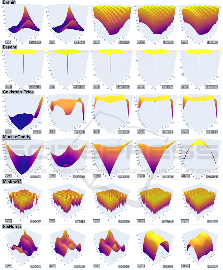
Figure 2: The three evolutionary patterns for the objective landscapes in this study are global minimum narrowing which
is seen in Easom only, ruggedness increase (or increase in number of local minima) which is seen in Mishra04 only, and a
concave-to-convex inversion which is seen in Goldstein-Price and Six-Hump Camel (and in Branin and Martin-Gaddy which
are not depicted).
Making Hard(Er) Bechmark Test Functions
35

Figure 3: Mean objective deficiency (MOD
100
), or ‘hardness’ of the six evolved objective landscapes.
seen. The derivative function then needs to be con-
tinuous under all possible parameterizations, and cal-
culated in every function evaluation which might be
computationally expensive. The alternative, analyz-
ing the hardness after evolution only, comes with the
risk of not being feasible or representative. In any
case, for evolved objective landscapes to be actually
usable as benchmarks, we need exact values for min-
ima, maxima, and their coordinates.
A second noteworthy point is the manipulation of
scalar constants as we chose them. We tried to in-
corporate every logically mutable factor and addition
in the process, but also made some arbitrary deci-
sions in the process, like not including powers. The
example of Section 5, f (x) = cos(x) and its equiva-
lent f (x) = 1 ·cos(1 ·x + 0) + 0, can also be seen as
f (x) = 1 ·cos(1 ·x
1
+ 0)
1
+ 0 (notice the change from
x to x
1
). Leaving these out as we did surely excludes
a wide range of possible formulae and their accompa-
nying objective landscapes. It might take some time,
thinking and discussion to determine the most generic
yet feasible way of navigating the state space of possi-
ble functions. Apart from this, raising the caps might
also help, but also allows for wilder functions and ex-
treme ranges, unsuitable for testing evolutionary al-
gorithms.
Third, it is important to discuss the possibilities of
local maxima in the evolutionary process itself. The
used benchmark evolver is basically a stochastic hill-
Climber. While enjoying the advantage of being easy
to use and requiring no hyperparameters, hillClimbers
are known to get stuck in local maxima. So in a
slightly paradoxical way, the algorithm that makes
landscapes harder by creating local minima is prone
to getting trapped in local minima itself. Possible so-
lutions might incorporate the use of variable mutation
strength, simulated annealing (Dahmani et al., 2020)
or maybe even a population based algorithm as a func-
tion evolver.
Fourth and finally, the most obvious improvement
might be widening the scope of functionality and di-
mensionality. Performing more or longer runs is a
good idea because as we stand, we have no idea
whether these hits are incidental or more structural. In
a more ambitious fashion, we could try to evolve the
entire function structure instead of the scalars only.
This will result in new developmental problems, such
as division by zero, or negative numbers in logarithms
and square roots. But new problems will have new
solutions, and we must find them to ensure continuity
in navigation the evolutionary landscape. An inter-
mediate solution would be to explore the possibility
of tuning the benchmark generators mentioned in the
introduction with an evolutionary algorithm. In any
case, upscaling this experiment in any of these direc-
tions like leads to new results.
Contemplating these results, the echoes of the no
free lunch theorem still resound through the valleys of
objective landscapes, reminding us that at this point,
the evolved hard objective landscapes are necessarily
hard for the plant propagation only. No free lunch
means we are fitting problem (instance)s to optimiza-
tion algorithms and as such, we could ultimately just
be uncovering the intricate interplay between both.
REFERENCES
Anonymous (2022). Repostory containing source material
for this study.
Applegate, D., Bixby, R., Chvatal, V., and Cook, W. (1999).
Finding tours in the tsp. Technical report.
Bartz-Beielstein, T., Doerr, C., Bossek, J., Chandrasekaran,
S., Eftimov, T., Fischbach, A., Kerschke, P., L
´
opez-
ECTA 2022 - 14th International Conference on Evolutionary Computation Theory and Applications
36

Ib
´
a
˜
nez, M., Malan, K. M., Moore, J. H., Naujoks, B.,
Orzechowski, P., Volz, V., Wagner, M., and Weise, T.
(2020). Benchmarking in Optimization: Best Practice
and Open Issues. arXiv, pages 1–50.
Braam, F. and van den Berg, D. (2022). Which rectangle
sets have perfect packings? Operations Research Per-
spectives, page 100211.
Brouwer, N., Dijkzeul, D., Koppenhol, L., Pijning, I., and
Van den Berg, D. (2022). Survivor selection in a
crossoverless evolutionary algorithm. In Proceedings
of the 2022 Genetic and Evolutionary Computation
Conference Companion. (in press).
Brownlee, J. et al. (2007). A note on research methodol-
ogy and benchmarking optimization algorithms. Com-
plex Intelligent Systems Laboratory (CIS), Centre for
Information Technology Research (CITR), Faculty of
Information and Communication Technologies (ICT),
Swinburne University of Technology, Victoria, Aus-
tralia, Technical Report ID, 70125.
Dahmani, R., Boogmans, S., Meijs, A., and Van den Berg,
D. (2020). Paintings-from-polygons: Simulated an-
nealing. In ICCC.
De Jonge, M. and van den Berg, D. (2020). Parameter sen-
sitivity patterns in the plant propagation algorithm. In
IJCCI, page 92–99.
de Jonge, M. and van den Berg, D. (2020). Plant propa-
gation parameterization: Offspring & population size.
Evo* 2020, page 19.
Dijkzeul, D., Brouwer, N., Pijning, I., Koppenhol, L., and
Van den Berg, D. (2022). Painting with evolutionary
algorithms. In International Conference on Compu-
tational Intelligence in Music, Sound, Art and Design
(Part of EvoStar), pages 52–67. Springer.
Doerr, C., Ye, F., Horesh, N., Wang, H., Shir, O. M., and
B
¨
ack, T. (2020). Benchmarking discrete optimization
heuristics with iohprofiler. Applied Soft Computing,
88:106027.
Fraga, E. S. (2019). An example of multi-objective opti-
mization for dynamic processes. Chemical Engineer-
ing Transactions, 74:601–606.
Gallagher, M. and Yuan, B. (2006). A general-purpose tun-
able landscape generator. IEEE transactions on evo-
lutionary computation, 10(5):590–603.
Geleijn, R., van der Meer, M., van der Post, Q., and van den
Berg, D. (2019). The plant propagation algorithm on
timetables: First results. EVO* 2019, page 2.
Haddadi, S. (2020). Plant propagation algorithm for nurse
rostering. International Journal of Innovative Com-
puting and Applications, 11(4):204–215.
Iori, M., De Lima, V., Martello, S., and M., M. (2021a).
2dpacklib: a two-dimensional cutting and packing li-
brary (in press). Optimization Letters.
Iori, M., de Lima, V. L., Martello, S., Miyazawa, F. K., and
Monaci, M. (2021b). Exact solution techniques for
two-dimensional cutting and packing. European Jour-
nal of Operational Research, 289(2):399–415.
Iori, M., de Lima, V. L., Martello, S., and Monaci, M.
(2021c). 2dpacklib.
Kerschke, P. and Trautmann, H. (2019). Comprehen-
sive feature-based landscape analysis of continuous
and constrained optimization problems using the r-
package flacco. In Applications in Statistical Com-
puting, pages 93–123. Springer.
Koppenhol, L., Brouwer, N., Dijkzeul, D., Pijning, I.,
Sleegers, J., and Van den Berg, D. (2022). Survivor
selection in a crossoverless evolutionary algorithm.
In Proceedings of the 2022 Genetic and Evolutionary
Computation Conference Companion. (in press).
Laguna, M. and Marti, R. (2005). Experimental testing of
advanced scatter search designs for global optimiza-
tion of multimodal functions. Journal of Global Opti-
mization, 33(2):235–255.
Lou, Y., Yuen, S. Y., and Chen, G. (2018). Evolving bench-
mark functions using kruskal-wallis test. In Proceed-
ings of the Genetic and Evolutionary Computation
Conference Companion, pages 1337–1341.
Malan, K. M. and Engelbrecht, A. P. (2013). A survey of
techniques for characterising fitness landscapes and
some possible ways forward. Information Sciences,
241:148–163.
Paauw, M. and Van den Berg, D. (2019). Paintings,
polygons and plant propagation. In International
Conference on Computational Intelligence in Music,
Sound, Art and Design (Part of EvoStar), pages 84–
97. Springer.
Pohlheim, H. (2007). Examples of objective functions. Re-
trieved, 4(10):2012.
Reinelt, G. (1991). Tsplib—a traveling salesman problem
library. ORSA journal on computing, 3(4):376–384.
Rice, J. R. (1976). The algorithm selection problem. In Ad-
vances in computers, volume 15, pages 65–118. Else-
vier.
Rodman, A. D., Fraga, E. S., and Gerogiorgis, D. (2018).
On the application of a nature-inspired stochastic
evolutionary algorithm to constrained multi-objective
beer fermentation optimisation. Computers & Chemi-
cal Engineering, 108:448–459.
Salhi, A. and Fraga, E. S. (2011). Nature-inspired optimi-
sation approaches and the new plant propagation algo-
rithm.
Selamo
˘
glu, B.
˙
I. and Salhi, A. (2016). The plant propaga-
tion algorithm for discrete optimisation: The case of
the travelling salesman problem. In Nature-inspired
computation in engineering, pages 43–61. Springer.
Sleegers, J. and Berg, D. v. d. (2021). Backtracking (the)
algorithms on the hamiltonian cycle problem. arXiv
preprint arXiv:2107.00314.
Sleegers, J. and van den Berg, D. (2020a). Looking for
the hardest hamiltonian cycle problem instances. In
IJCCI, pages 40–48.
Sleegers, J. and van den Berg, D. (2020b). Plant propaga-
tion & hard hamiltonian graphs. Evo* 2020, page 10.
Smith-Miles, K., Hemert, J. v., and Lim, X. Y. (2010). Un-
derstanding tsp difficulty by learning from evolved in-
stances. In International conference on learning and
intelligent optimization, pages 266–280. Springer.
Socha, K. and Dorigo, M. (2008). Ant colony optimization
for continuous domains. European journal of opera-
tional research, 185(3):1155–1173.
Making Hard(Er) Bechmark Test Functions
37

Suganthan, P. N., Hansen, N., Liang, J. J., Deb, K., Chen,
Y.-P., Auger, A., and Tiwari, S. (2005). Problem defi-
nitions and evaluation criteria for the cec 2005 special
session on real-parameter optimization. KanGAL re-
port, 2005005(2005):2005.
Sulaiman, M., Salhi, A., Fraga, E. S., Mashwani, W. K., and
Rashidi, M. M. (2016). A novel plant propagation al-
gorithm: modifications and implementation. Science
International, 28(1):201–209.
Sulaiman, M., Salhi, A., Khan, A., Muhammad, S., and
Khan, W. (2018). On the theoretical analysis of the
plant propagation algorithms. Mathematical Problems
in Engineering, 2018.
van Hemert, J. I. (2006). Evolving combinatorial problem
instances that are difficult to solve. Evolutionary Com-
putation, 14(4):433–462.
van Horn, G., Olij, R., Sleegers, J., and van den Berg, D.
(2018). A predictive data analytic for the hardness of
hamiltonian cycle problem instances. Data Analytics,
2018:101.
Vrielink, W. and van den Berg, D. (2019). Fireworks algo-
rithm versus plant propagation algorithm. In IJCCI,
pages 101–112.
Vrielink, W. and van den Berg, D. (2021a). A dynamic
parameter for the plant propagation algorithm. Evo*
2021, pages 5–9.
Vrielink, W. and van den Berg, D. (2021b). Parameter con-
trol for the plant propagation algorithm. Evo* 2021,
pages 1–4.
Weise, T., Li, X., Chen, Y., and Wu, Z. (2021). Solving
job shop scheduling problems without using a bias
for good solutions. In Proceedings of the Genetic
and Evolutionary Computation Conference Compan-
ion, pages 1459–1466.
Weise, T. and Wu, Z. (2018a). Difficult features of com-
binatorial optimization problems and the tunable w-
model benchmark problem for simulating them. In
Proceedings of the Genetic and Evolutionary Compu-
tation Conference Companion, pages 1769–1776.
Weise, T. and Wu, Z. (2018b). The tunable w-model bench-
mark problem.
Wolpert, D. H. and Macready, W. G. (1997). No free lunch
theorems for optimization. IEEE transactions on evo-
lutionary computation, 1(1):67–82.
ECTA 2022 - 14th International Conference on Evolutionary Computation Theory and Applications
38
