Fast Algorithms for the Capacitated Vehicle Routing Problem using

Machine Learning Selection of Algorithm’s Parameters

Roberto As

ın-Ach

1 a

, Olivier Goldschmidt

2 b

, Dorit S. Hochbaum

3 c

and Isa

ıas I. Huerta

1 d

Department of Computer Science, Universidad de Concepci

on, Chile

Riverside County Ofﬁce of Education, U.S.A.

Department of Industrial Engineering and Operations Research, University of California, Berkeley, U.S.A.

Keywords:

Vehicle Routing, Machine Learning, Model Selection.

Abstract:

We present machine learning algorithms for automatically determining algorithm’s parameters for solving

the Capacitated Vehicle Routing Problem (CVRP) with unit demands. This is demonstrated here for the

“sweep algorithm” which assigns customers to a truck, in a wedge area of a circle of parametrically selected

radius around the depot, with demand up to its capacity. We compare the performance of several machine

learning algorithms for the purpose of predicting this threshold radius parameter for which the sweep algorithm

delivers the best, lowest value, solution. For the selected algorithm, KNN, that is used as an oracle for the

automatic selection of the parameter, it is shown that the automatically conﬁgured sweep algorithm delivers

better solutions than the “best” single parameter value algorithm. Furthermore, for the real worlds instances

in the new benchmark introduced here, the sweep algorithm has better running times and better quality of

solutions compared to that of current leading algorithms. Another contribution here is the introduction of the

new CVRP real world data benchmark based on about a million customers locations in Los Angeles and about

a million customers locations in New York city areas. This new benchmark includes a total of 46000 problem

instances.

1 INTRODUCTION

The Capacitated Vehicle Routing Problem (CVRP) is

a well known NP-hard problem that has been exten-

sively studied due to its importance in applications in

logistics and transportation. An instance of this prob-

lem consists of a depot, where trucks are located, and

a distribution of customers and their demands. The

goal is to devise tours for trucks that visit the cus-

tomers and deliver their demands, subject to the given

truck capacity, and so that the sum of distances tra-

versed by the trucks is minimum. A large number of

exact and heuristic algorithms have been devised for

the CVRP. In addition to algorithms, there are also

multiple benchmarks of data sets that are available for

the purpose of testing algorithms for CVRP. These in-

clude synthetic and real world data and consist mostly

of small instances (with fewer than 1000 customers).

https://orcid.org/0000-0002-1820-9019

https://orcid.org/0000-0002-6727-5565

https://orcid.org/0000-0002-2498-0512

https://orcid.org/0000-0002-0343-4539

One exception is the Gendreau benchmark (Arnold

et al., 2019) that includes large instances of size up

to 30000.

In general, when there are several algorithms to

solve a problem, no single algorithm dominates the

others on all problem instances. Algorithm selection

attempts to build machine-learning-based oracles ca-

pable of determining, in advance, which algorithm

can perform best for a given input instance. Simi-

larly, for a single algorithm, several conﬁgurations of

the algorithm are possible (i.e. different values for the

algorithm’s parameters). Again, it is often the case

that no single conﬁguration performs best on all pos-

sible scenarios. Algorithm Conﬁguration is the task

of building machine-learning-based oracles that can

output the best conﬁguration for a given instance.

In this work we present a case study for automatic

algorithm conﬁguration for the “Sweep Algorithm”.

The sweep algorithm assigns customers to a truck, in

a wedge area of a circle of parametrically selected ra-

dius around the depot, with demand up to the truck ca-

pacity. This radius parameter affects the output of the

algorithm, and its best value depends on an instance

Asín-Achá, R., Goldschmidt, O., Hochbaum, D. and Huerta, I.

Fast Algorithms for the Capacitated Vehicle Routing Problem using Machine Learning Selection of Algorithm’s Parameters.

DOI: 10.5220/0011405400003335

In Proceedings of the 14th International Joint Conference on Knowledge Discovery, Knowledge Engineering and Knowledge Management (IC3K 2022) - Volume 1: KDIR, pages 29-39

ISBN: 978-989-758-614-9; ISSN: 2184-3228

characteristics. In our study, we propose and com-

pare several Machine Learning (ML) algorithms for

identifying the appropriate parameter for each input

instance. We compare the algorithms’ performance

with the Single Best Solver (i.e. the by-default best

parameter value across all the instances) and the Vir-

tual Best Solver (i.e. a perfect solver that identiﬁes the

best parameter value for each instance without over-

head).

Our contributions here include:

• The generation of new benchmark sets based on

real world addresses in New York and Los Ange-

les cities. With our instance generator, one can

generate random subset instances of sizes up to

one million customers.

• An automatically selected algorithm that gener-

ates very fast feasible solutions, which, when

compared to the ﬁrst solutions found by OR

tools (Perron and Furnon, 2019) public solver, and

by the state-of-the-art FILO solver, publicly avail-

able, solver from (Accorsi and Vigo, 2021), de-

liver better quality solutions in dramatically faster

running times.

• Demonstrating the feasibility of building

machine-learning-based oracles capable of iden-

tifying a “best” parameter value of an algorithm,

resulting in considerable speed up and improved

solution quality.

The paper is structured as follows: Section 2

presents the basic concepts and terminology used in

the rest of the paper. It also presents relevant related

work in the ﬁeld. In Section 3, we present and elabo-

rate on our automatically conﬁgured sweep algorithm.

Experimental results are presented in Section 4. Sec-

tion 5 includes conclusions and pointers to future re-

search.

2 PRELIMINARIES AND

RELATED WORK

2.1 The Capacitated Vehicle Routing

Problem and Algorithms

In the Capacitated Vehicle Routing Problem (CVRP)

there is a set of customers with known demands and

an unlimited collection of trucks, of limited capacity,

located at the “depot” which are to deliver the goods

to the customers so as to satisfy their demands. A

solution to the problem is a set of routes for the trucks,

such that each route begins and ends at the depot, the

total demand is satisﬁed, and no truck’s capacity is

exceeded. The goal is to minimize the sum of the

lengths of the tours traversed by all the trucks.

CVRP is a well known NP-hard problem, which

generalizes the Travelling Salesperson Problem. Due

to its difﬁculty, and its importance in applications, a

large number of algorithms were devised for CVRP,

most of which are heuristic algorithms that do not

guarantee optimality. A recent review of such algo-

rithms is provided in (Elshaer and Awad, 2020). Ex-

act algorithms have also been proposed for the prob-

lem, one of which, (Pessoa et al., 2021), is considered

particularly inﬂuential. Recently, Machine-Learning-

based heuristics have been proposed, mostly for

small-size problem instances (Bogyrbayeva et al.,

2022; Alesiani et al., 2022; Fellers et al., 2021).

Recall that we address here CVRP with unit

demands–that is, all customers demands are equal to

1 unit.

2.2 Our Sweep Algorithm

implementation

The sweep algorithm (Haimovich and Rinnooy Kan,

1985; Dondo and Cerd

a, 2013; Gillett and Miller,

1974) consists of two phases. In the ﬁrst phase cus-

tomers are allocated to trucks and in the second phase

a short route for each truck is computed, starting

from the depot, serving its customers, and returning

to the depot. The second phase can use any Travelling

Salesperson Problem (TSP) algorithm. In our imple-

mentation we solve the TSP using the Lin-Kernigan

(Lin and Kernighan, 1973) heuristic, as implemented

in the Concorde (Applegate et al., 2009) package, in

C language.

The ﬁrst phase of the sweep algorithm, in which

customers are allocated to trucks, consists of two sub-

phases:

1. Customers are partitioned into two groups. The

ﬁrst group consists of the customers which are

within a given distance parameter, radius, from

the depot. The remaining customers form the sec-

ond group.

2. In each group:

(a) With respect to the depot, compute the polar

coordinates of each customer and sort the cus-

tomers by increasing angle to the depot.

(b) One by one, assign the sorted customers such

that the total demand of customers assigned to

a truck doesn’t exceed the truck capacity. Note

that customers allocated to a truck in the ﬁrst

group are located in a wedge of the circle cen-

tered at the depot, see Figure 1.

KDIR 2022 - 14th International Conference on Knowledge Discovery and Information Retrieval

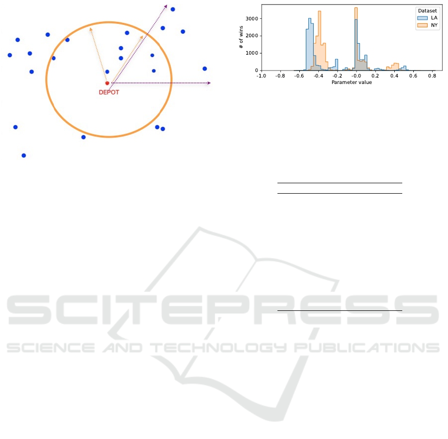
Figure 1: For the case of truck capacity 4 and unit demands,

this ﬁgure illustrates an inner wedge and an outer wedge for

the sweep algorithm.

In the special case of unit demands, we also im-

plement a variation of the sweep algorithm where the

total number of customers in the outer circle is an in-

teger multiple of the truck capacity. In case the se-

lected radius is such that the number of customers on

the outer circle is not an integer multiple of the truck

capacity, we move the extra customers to the inner cir-

cle by effectively increasing the radius. The rationale

behind this is to avoid sending a truck serving fewer

customers than its capacity far from the depot. This

variation is referred as the second algorithm.

The Sweep Algorithm’s Parameter: We will use the

“radius” parameter r, which is computed as the ratio

of the radius of the inner circle divided by the distance

to the furthest customer from the depot. This param-

eter r takes values in the range [0, 1]. We use negative

values of r to indicate the use of the second algorithm

with the parameter |r|.

Figure 2 shows the number of instances that are

“best” solved by a given parameter value for the LA

and NY benchmark sets (to be discussed in Subsec-

tion 3.2.1). This ﬁgure implies that, on average, the

second variant of the algorithm performs better than

the ﬁrst. Furthermore there is no uniform “best” pa-

rameter for all instances. Therefore, the prediction on

a “best” parameter value for a given instance is non

trivial and we will show that it can successfully be

done with machine learning methods.

We further note, from the results in Figure 2, that

the dominant best parameter values depend on the

benchmark set (NY or LA).

Overall, Table 1 lists the ﬁrst 10 parameter values

that perform best. We observe that parameter value

0 seems to work best, with values close to −0.5 (i.e.

−0.49, −0.4, −0.51, −0.42, −0.39, −0.48, −0.41,

−0.43) performing next best. We use this list of pa-

Figure 2: Number of instances which are best solved by

parameter value.

rameter values when evaluating the effectiveness of

the oracle, in Section 4.

Table 1: List of best 10 parameter values ordered according

to the percentage of best solved instances.

Parameter Value r % Wins

0 14.58

−0.5 4.09

−0.49 4.04

−0.4 3.72

−0.51 3.4

−0.42 3.36

−0.39 3.33

−0.48 3.32

−0.41 3.22

−0.43 2.92

Figures 3 and 4 show how the normalized cost (i.e.

the length of the tour normalized by dividing it by the

best (minimal) known value of each instance) varies

for different values of the parameter. Figure 3 shows

one line for the median value of all instances grouped

by different truck capacity. Besides observing that

the value can vary signiﬁcantly for close parameter

values, particularly for the ﬁrst algorithm), we also

notice that the trend is different depending on the ca-

pacity of the trucks. For instance, we can see that the

best value for instances for large capacities are among

the worst values for instances with small capacities.

We observe that the difference between “best” and

“worst” parameter values correspond to a magnitude

that is around 14% of the value of the “best solution”.

The behavior for the parameters corresponding to the

second algorithm is different than the one for the ﬁrst

algorithm due to the effect of the “padding” of the

outer circle customers to multiples of the truck capac-

ity, since many close values deliver exactly the same

solution.

Analogously, Figure 4 shows one line for the me-

dian values of all instances grouped by number of cus-

tomers. Again, we notice that close parameter values

in the ﬁrst algorithm can generate solutions of very

different quality. Here, we see that the normalized

difference between best and worse solutions can scale

Fast Algorithms for the Capacitated Vehicle Routing Problem using Machine Learning Selection of Algorithm’s Parameters

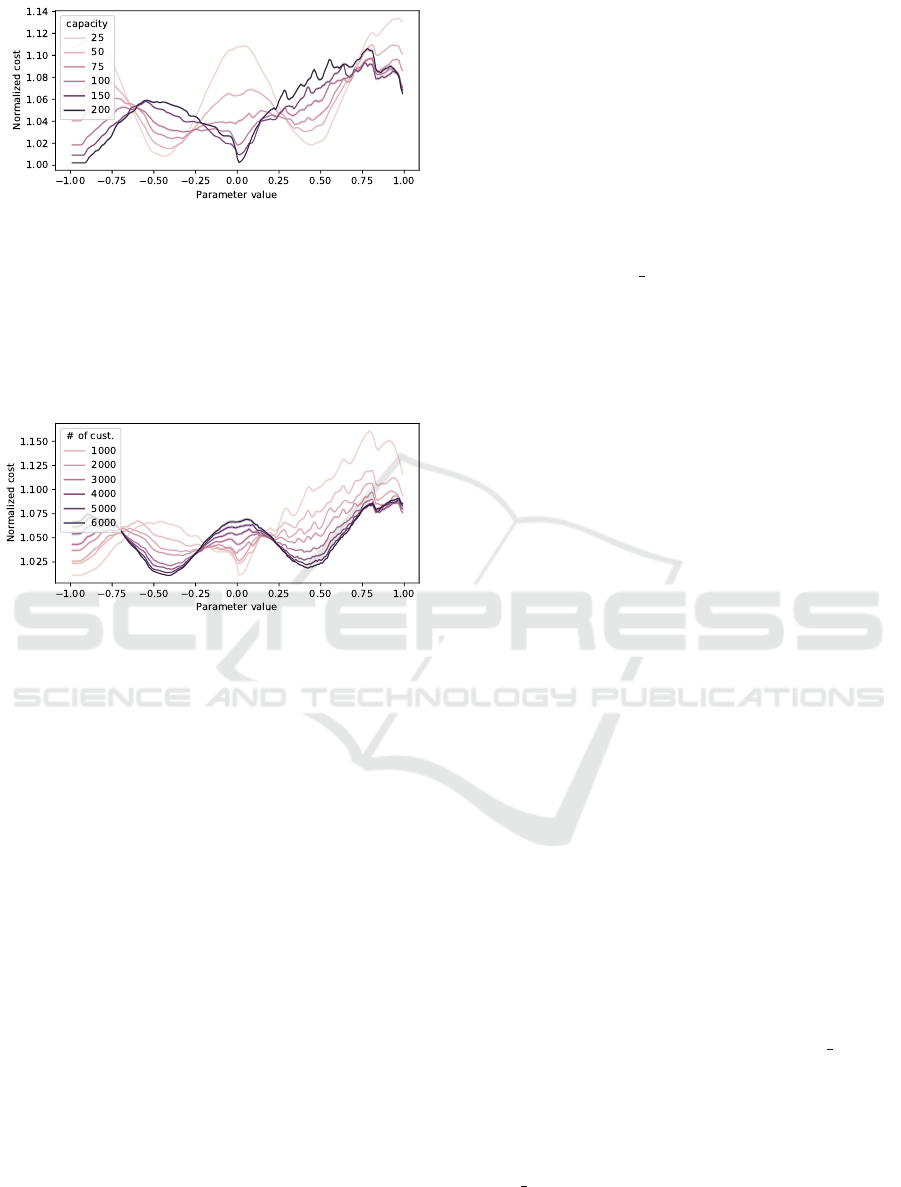
Figure 3: Normalized mean cost variation across possible

parameter’s values by truck capacity of all 46000 instances.

up to 15%. As in the previous case, the trend of the

normalized cost across the different parameter values

varies depending on the number of clients. For ex-

ample, we can see that good parameter values for big

instances are among the worse parameter values of the

smaller ones.

Figure 4: Normalized mean cost variation across possible

parameter’s values by number of customers of al 46000 in-

stances.

2.3 Machine Learning

Machine Learning (ML) is an Artiﬁcial Intelligence

ﬁeld that has seen huge development during the last

decade (Alpaydin, 2021). It is considered one of the

most powerful tools for processing and analyzing big

data volumes. Algorithms proposed for the differ-

ent ML models seek to identify hidden patterns in

the data, from which they can learn. In general, ML

models seek to learn, from given data, called train-

ing set, a function f that maps an input instance to

a corresponding scalar (vector) output, referred to as

label(s). ML models can be classiﬁed based on how

f is learned. When the learning process is based on

the use of ground truth, consisting of a set of input in-

stances and the associated correct output labels (dis-

crete or continuous), then the model is known as su-

pervised, e.g. (Burkart and Huber, 2021). When la-

bels are not available, the model ﬁnds patterns by an-

alyzing the nature of the input data, then the model is

said to be unsupervised, e.g. (Alloghani et al., 2020).

If the learning process of the model is based on both

ground-truth data and pattern analysis of the input

data, then it is known as semi-supervised, e.g. (Zhu

and Goldberg, 2009).

We also classify ML models depending on the na-

ture of the output of the mapping f . If the output

assumes discrete values, known as “classes”, that are

used to separated the possible inputs on different cate-

gories, the model is said to be a classiﬁcation model.

If the output is given as real (ﬂoating-point) values,

then the model is called a regression model.

The ML algorithms used here are:

Random Forests (RF) (Breiman, 2001): is an en-

semble method (Breiman, 1996) that constructs a

parameterized (n estimators) number of decision

trees (Quinlan, 1986), that are trained, each one,

with a different subset of instances belonging to

the training set. To compute the output label, each

of the trees “proposes” a result. The ﬁnal result

is determined by a consensus scheme that varies

depending if the model is a regression or a clas-

siﬁcation one. In the regression case, the consen-

sus corresponds to the average of all the decision

trees’ outputs, while for the classiﬁcation version,

the ﬁnal output corresponds to the label that re-

peats (is voted) the most, among the trees’ out-

puts.

k-Nearest Neighbors (KNN) (Fix and Hodges,

1989): is a ML algorithm that bases the output

label on the labels of the k closest training

examples to the input point we want to label.

Although several distance metrics can be used,

the euclidean distance between feature vectors

is the most common one. For classiﬁcation

tasks, KNN assigns the output label as the most

repeated label among the k neighbors. In case

of a regression task, the label corresponds to the

average of the labels of the k neighbors.

Ada Boost (AB) (Schapire, 2013): belongs to a

class of ensemble methods known as boost-

ing (Schapire, 1997). This technique consists on,

iteratively, reﬁning the “weakest model” in the en-

semble (e.g. a decision tree). First, this model

is trained with the complete training set, then a

higher weight is assigned to the data points which

accumulate bigger deviations on the metric being

optimized (e.g. the error). The weights are com-

puted from a parameter called learning rate. A

new iteration with another “weak” model is per-

formed using the new weights from the previous

step, in order to correct the highest deviations of

the previous model. This is repeated for a num-

ber of iterations which is given as a parameter

(n estimators).

Gradient Boosting (GB) (Friedman, 2001): is also

a boosting model that generalizes the ideas be-

KDIR 2022 - 14th International Conference on Knowledge Discovery and Information Retrieval

hind Ada Boost. For it, different parameterized

loss functions can be deﬁned. For the learn-

ing, the model, consecutively, learns a parameter-

ized number (n estimators) of new “weak” mod-

els that are given as input to the next iteration.

For each new model, in a similar way of gradi-

ent descent, a negative gradient is computed based

on the past model which is weighted according

to a parameterized scheme (learning rate), and

a move in the opposite direction for reducing the

loss is performed.

Convolutional Neural Networks(CNN)

(Fukushima and Miyake, 1982): are a spe-

cial type of Neural Networks (McCulloch and

Pitts, 1943) that specialize in processing topo-

logical data in form of matrices (i.e. an image).

Its structure is typically composed by three types

of layers: convolutional layer, pooling layers

and fully connected layers. The main operation

of this kind of networks is that of convolution

consisting of computing the dot product between

two matrices: a submatrix of the input matrix

and another matrix called kernel (also called

ﬁlter). The kernel contains parameters that are

learnt during the training phase. The result of

performing several convolutions of the image

is a new set of features that is fed to the next

layer, which in turn corresponds to high level

characteristics of the input data (e.g. borders,

corners, colors, etc). The pooling layers are used

in order to reduce the dimensionality of each

feature map resulting of the convolution phase.

This is done by performing single operations over

the matrices like obtaining the maximum or the

average of its values. This way, each matrix is

“compressed” into one single value that is later

fed to the fully connected layers, which usually

correspond to the last layers of the network.

These layers map this “compressed data” into

the corresponding output of the model (i.e. the

labels).

2.4 Per Instance Automatic Algorithm

Conﬁguration

According to (Kerschke et al., 2019), automatic al-

gorithm conﬁguration consists of determining the pa-

rameter values of a given algorithm (its conﬁgura-

tion) in order to optimize its average performance

across the instances of a given benchmark set. Per-

instance algorithm conﬁguration is a generalization

of this problem, where the conﬁguration is optimized

for a speciﬁc input instance. For the latter, we can

identify two phases: a training phase, where the per-

instance conﬁgurator learns from the characteristics

and performance metrics of known training instances,

for which training set labels exist, and a production

phase where it is used to select the best conﬁguration

for a given, new, instance. In contrast, (per-set) au-

tomatic algorithm conﬁguration (see (L

opez-Ib

nez

et al., 2016)) sets “good average” values that are used

for all the test instances, once it is trained. One ap-

proach for Per-instance algorithm conﬁguration is to

consider it as an special case of automatic algorithm

selection (Lindauer et al., 2015), where a ﬁnite num-

ber of different conﬁgurations correspond to a ﬁnite

number of algorithms, and the task consists on ﬁnd-

ing which, among such conﬁgurations, would per-

form best in a given input instance (Rice, 1976). For-

mally, as deﬁned in (Lindauer et al., 2019), the goal is

to select, for a given instance and a given metric m, an

algorithm A, whose performance metric value is best.

Previous work on algorithm selec-

tion/conﬁguration for CVRP, include (Fellers

et al., 2021), where the authors present a CNN-based

meta-solver that is capable of identifying, from a set

of 4 heuristic algorithms, for up to 79% of instances,

the one that performs best, in a set of diverse in-

stances automatically generated by the authors. The

instances considered in such study vary the number

of customer in the range [100 − 1000]. Also, a recent

survey on learning-based algorithms for the CVRP

can be found in (Bogyrbayeva et al., 2022).

2.5 Performance Metrics

To evaluate algorithm selection methods, two base-

lines are frequently used:

Single Best Solver (SBS): relates to the perfor-

mance of the solver with best average behavior

across all the instances used for the ﬁrst phase

(i.e. the best solver on average for the training

set).

Virtual Best Solver (VBS): relates to a virtual

solver that delivers perfect selection of the

best performing algorithm for each individual

instance.

An algorithm selector is reasonable if it performs

at least as well as the SBS. Hence, it is common to

normalize the performance metric m with respect to

this baselines. For this problem, we take m as the

length of all trucks’ tours. This normalized metric is

known as ˆm and is deﬁned as follows:

ˆm =

m − m

V BS

SBS

− m

V BS

(1)

Values of ˆm = 0 mean that the selector performs

as well as the VBS and ˆm = 1 means that it performs

Fast Algorithms for the Capacitated Vehicle Routing Problem using Machine Learning Selection of Algorithm’s Parameters

as well as the SBS. Greater than 1 values of ˆm mean

that the use of the selector is worse than using a sin-

gle algorithm/conﬁguration for all the instances in the

test.

For evaluating the performance of different ML

models on the quality of the predicted parameter r,

we use the Mean Squared Error (Carbone and Arm-

strong, 1982) (MSE). This measures the average of

the squares of the differences between the predicted

values of r and the best possible values of r. This best

value is determined for each instance by running all

possible values of r and picking the one which gives

the lowest value of the length of the tours. This best

value is referred to as the ground-truth label of the

instance.

3 META-SWEEP-ALGORITHM:

AUTOMATIC

CONFIGURATION OF THE

SWEEP ALGORITHM

3.1 Algorithm Conﬁguration as

Algorithm Selection

As proposed in (Lindauer et al., 2015), algorithm con-

ﬁguration tasks can be handled the same way as algo-

rithm selection tasks. For this, typically, a continu-

ous domain has to be discretized and bounded. For

the Sweep Algorithm, this is straightforward, since

its parameter is bounded by the range [0, 1] and such

a range can be discretized at a desired level of gran-

ularity. The algorithm selector setup for the Sweep

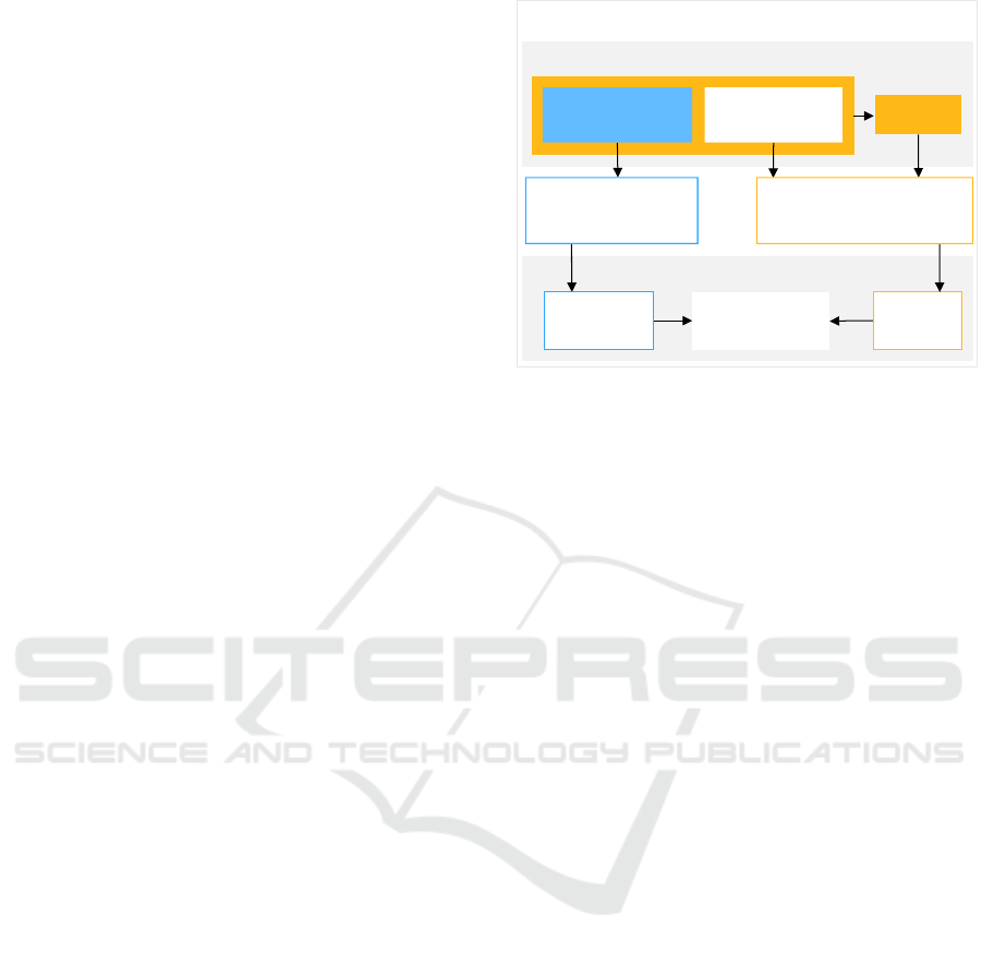
algorithm is given in Figure 5.

The process is composed of the following tasks:

Training and Testing Data Preparation: For this

task, benchmark sets have to be collected, and all

possible conﬁgurations of the algorithm have to

be tested against those benchmark sets. For each

experiment, the cost obtained by the algorithm

and the time of the execution is stored.

Instance Characterization: The instances are char-

acterized by devising and selecting a set of fea-

tures that are ideally informative. It is also impor-

tant that computation of the features of an instance

is done efﬁciently, since the focus of algorithm se-

lection is low running time overall.

Instance Labeling: Since our approach here is su-

pervised, we need to label our training set. These

labels are computed by comparing the quality of

the costs of the solutions associated to the corre-

sponding parameter values.

Instances

Parameter

values

Instance

Characterization

Supervised

model

Costs

Input Output

Training and testing data preparation

Machine Learning Training

Instance labeling

Algorithm configuration framework

Figure 5: Training process for our supervised algorithm

conﬁguration framework.

Machine Learning Models: A machine learning

model is deﬁned by its input, output and the

function that maps the input into the output.

The input consists of the (possibly normalized)

features determined in the characterization step

above and the output corresponds to the (possibly

normalized) labels also described above. The

learning of the mapping is then computed by

ML algorithms that adjust the parameters of

the underlying structure of the model (neural

network, decision trees, etc). After this, the

model is validated by comparing the model’s

output with the labels in the testing data.

Next, we elaborate on the details of each of the

tasks.

3.2 The Generated Training and Testing

Data

3.2.1 Los Angeles and New York Datasets

The customers of each instance are randomly selected

either from a set of over one million addresses in

Los Angeles, (https://data.lacity.org), or from a set

of close to one million addresses in New York City

(https://data.cityofnewyork.us). Each customer is de-

ﬁned by its latitude and longitude coordinates. The

distance between two customers is calculated as the

Euclidean distance. For each instance, we locate the

depot at the mid-point between the most south-west

and the most north-east customers.

In this study, we set all demands to unit. The num-

ber of customers per instance varies from 500 to 6000,

randomly selected, and the truck capacity varies from

25 to 200 customers. For every combination of num-

ber of customers and truck capacity, we have gener-

KDIR 2022 - 14th International Conference on Knowledge Discovery and Information Retrieval

ated 500 instances from each of the Los Angeles and

the New-York City collections of addresses. In total,

we generated 46000 instances.

3.3 Instance Characterization and

Features

Our models use different features of the CVRP in-

stances as input for suggesting the best conﬁguration

of the algorithm. Such features have to be informa-

tive and, hopefully, fast to compute. They are nor-

mally computed by preprocessing the input instance

and by extracting descriptive statistics from it. For

CVRP, fast to extract descriptive statistics are: num-

ber of customers, average and standard deviation of

the demands, statistics on the spatial distribution of

the customers, etc.

We choose the following features to feed to our

models:

Number of Customers. The total number of cus-

tomers in the CVRP problem.

Capacity: The capacity of the trucks. For this

work, we consider uniform capacity across all the

trucks, but this can easily be converted to a vector

of capacities if this is not the case.

Width. The biggest difference across x-coordinates

of all customers.

Height. The biggest difference across y-coordinates

of all customers.

k-circular Convolution. We take k-concentric cir-

cles, centered at the depot, in such a way that the

last circle has radius equivalent to the distance of

the depot to its furthest customer. The radius for

the other k − 1 circles are uniformly distributed

between the depot and the external circle. For

each circle i > 0 of radius r

, we compute the

percentage of customers that lie in the ﬂat donuts

formed by the circles of radius r

and r

i−1

. For

this work, we take k = 100.

Customers Matrix. This matrix is equivalent to the

one used in (Huerta et al., 2022): It is a 128× 128

matrix that is computed as follows. We uniformly

divide the euclidean space in which the customers

are disposed in a 128 × 128 layout and, for each

of the 16384 cells, we compute the number of cus-

tomers that are contained in the cell. For normal-

ization purposes, a top threshold value can be set

for really crowded cells.

The ﬁrst four features are used in all the models,

whereas k-circular convolution is used for RF, KNN,

AB and GB, and the customers matrix is used only for

CNN.

3.4 Instance Labeling

The instance labeling entails the computation of the

ground-truth label of each instance. As explained ear-

lier, this is the value of r that gives the best perfor-

mance of the Sweep algorithm for this instance. This

is given to the ML algorithms as the labels for the

training set.

3.5 Machine Learning Models Used

For training our regression model, we used several

ML algorithms. The parameters for the models were

adjusted using k-fold cross validation (Stone, 1974),

with k = 5. The results of this hyper-parameter tun-

ing and further details on each of the algorithms are

as follows:

Random Forests: n estimators = 510

k-Nearest Neighbors: k = 210

Gradient Boost: loss = MSE, learning rate = 0.1,

n estimators = 100.

Ada Boost: learning rate = 0.1, n estimators = 50.

Convolutional Neural Networks: The CNN is

formed by the following layers:

• 3 convolutional layers with 16,32 and 48, 3×3-

sized ﬁlters,

• 2 pooling layers of sizes 2 ×2,

• a dense layer of 32 nodes

• a layer that concatenates the previous layer with

the 4 features corresponding the number of cus-

tomers, capacity, width, height,

• 4 fully connected layers of sizes 512, 128, 32

and 10, the last one corresponding to the out-

put of the network.

All layers use the ReLu, a piece-wise linear ac-

tivation function (Agarap, 2018), with the excep-

tion of the last one, which uses a linear activation

function.

3.6 Meta-Sweep-Algorithm

The Meta-Sweep-Algorithm (MSA) is a per-instance

automatically conﬁgured algorithm. This meta-

algorithm ﬁrst computes the features, deﬁned in Sub-

section 3.3, associated with an input instance, which

are then fed to the selected machine-learning-based

oracle to predict the best parameter value. Then, the

meta-algorithm runs the sweep algorithm with this

predicted radius parameter.

Fast Algorithms for the Capacitated Vehicle Routing Problem using Machine Learning Selection of Algorithm’s Parameters

4 EXPERIMENTAL RESULTS

4.1 Comparing the Parameter

Prediction Quality of Different

Machine Learning Algorithms

The training and testing of the ﬁve ML algorithms

were performed on a machine with a 3.3Ghz AMD

Ryzen 9 5900HS processor with 16GB of RAM. A

Nvidia RTX 3060 GPU was also used for the training

of CNN. We used the Machine Learning Algorithms

implemented in the Scikit-learn and Keras (tensor-

ﬂow) modules of Python.

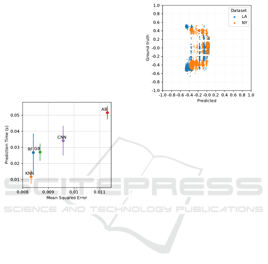
Figure 6: Quality (in terms of MSE) and running time com-

parison of ML algorithms.

Figure 6 shows the performance of the parame-

ter prediction of the ﬁve ML-algorithms. The per-

formance is measured in terms of MSE across the

training set and the running time (shown as mean and

standard deviation). As can be seen, GB and CNN

are the algorithms with largest MSE value. More-

over, for AB, the running time is the largest. KNN

delivers, on average, predictions of best quality and at

the fastest running time. RF and GB perform slightly

worse in quality, and take longer times (up to 3× the

time needed by KNN). Hence, for the rest of this sec-

tion, we report on results obtained by KNN.

In Figure 7 we contrast the ground-truth labels

with the predicted labels as computed by the KNN

algorithm. The ideal form of such graphic would be a

perfect diagonal, but we can observe chunks of values

for which the mislabeling is more common. For in-

stance, we notice that the algorithm predicts very dif-

ferent values when the ground-truth values are close

to 0. We also notice that the algorithm tends to predict

a negative value (i.e. the second algorithm) more of-

ten than when the real “best” parameter indeed corre-

Figure 7: Ground truth labels vs predicted labels by KNN.

sponds to the second algorithm. This may not have an

impact on the quality of the recommendation, since

there may be parameter values for the ﬁrst and sec-

ond algorithms that generate very close solutions in

the quality of the tour length. How this mislabelling

affects the performance in the length of the resulting

tour length is explored in the next subsections.

4.2 Comparison with Other CVRP

Solvers

We compare the results of our Meta-Sweep-

Algorithm (MSA) with other state-of-the-art solvers.

Speciﬁcally, we compare with OR-tools CVRP

solver (Perron and Furnon, 2019) with its default

parameters’ values, and with the publicly available

FILO solver, described in (Accorsi and Vigo, 2021),

also with its default parameters’ values. The CVRP

OR-tools solver is a constraint Programming solver

that supports multiple CVRP formulations. The FILO

solver is based on Iterated Local Search, which im-

plements several already proposed and new neighbor-

hoods, which acceptance criterion is based on that of

Simulated Annealing, in order to continually diver-

sifying and exploiting different regions of the search

space. More importantly for this work, FILO’s local

search initialize with the solution obtained by a C++

implementation of the classic Savings heuristic for the

VRP (Clarke and Wright, 1964), which we label CW.

For each of the 15333 instances in the testing set

(a third of the benchmark set), we run the three algo-

rithms: MSA, CW and OR-Tools. Figure 8 illustrates

the difference in the performances of the algorithms.

In this ﬁgure, each instance is presented as a point for

each of the three algorithms in blue (MSA), orange

(OR-Tools) and green (CW). The horizontal x-axis is

the computation time (in log-scale) taken by the algo-

KDIR 2022 - 14th International Conference on Knowledge Discovery and Information Retrieval

rithms to produce a ﬁrst solution. The vertical y-axis

is the solution quality measured as the ratio of the so-

lution value divided by the best value delivered by one

of the three algorithms.

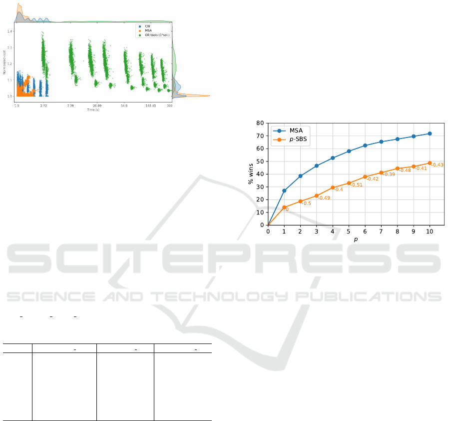
Figure 8: Time and quality comparison of MSA, OR-tools

and CW algorithms.

As can be seen, compared to OR-Tools, MSA

and CW produce better solutions and in dramatically

faster time. Compared to CW, MSA is noticeably

faster (on average 2x faster) and delivers most of the

best solutions computed. The gap between the solu-

tions both algorithms produce oscillates between very

small values and up to 18%. The most extreme vari-

ations seem to happen for the fastest-to-compute in-

stances, which are the smallest ones.

Table 2: Percentage of best solved instances per algo-

rithm and average runtime, grouped by number of cus-

tomers. # cust = number of customers. % MSA, % CW,

% OT = percentage of instances in the group best solved

by meta-sweep-algorithm, CW and OR-tools respectively,

and t MSA, t CW, t OT = average time needed to produce

the ﬁrst solution by meta-solver, CW and OR-tools respec-

tively, in seconds.

# cust. % MSA t MSA % CW t CW % OT t OT

500 82.89 0.03 17.11 0.02 0.0 1.77

1000 76.49 0.07 23.51 0.07 0.0 7.01

1500 75.68 0.11 24.32 0.13 0.0 15.61

2000 77.88 0.16 22.12 0.23 0.0 27.53

3000 73.76 0.23 26.24 0.5 0.0 61.43

4000 57.11 0.35 42.89 0.89 0.0 108.89

5000 56.93 0.44 43.07 1.4 0.0 169.41

6000 57.82 0.54 42.18 2.03 0.0 245.26

Table 2 reports the percentage of instances, out of

the 15333 instances, that are best solved by each of

the algorithms. It also shows the average time needed

by each algorithm to compute the solutions. This is

reported for each group of instances that share the

same number of customers. The results in this table

indicate that MSA ﬁnds solutions much faster than

the other algorithms–up to two orders of magnitude

faster than OR-Tools, and about a factor of 2 faster

than CW. Also, MSA ﬁnds better quality solutions for

most instances.

4.3 The Effectiveness of the KNN

Oracle

One way of evaluating the effectiveness of the oracle,

as proposed in (Dunning et al., 2018), is to make it

predict the best p values of r for each instance, and

compare them to a “single” best vector of values of

r for the entire dataset. This is a generalization of

the SBS as discussed in Section 2.5, which we call p-

SBS. For this, the model is trained to output not only

one, but the p best values of r. Here we set p = 10.

For SBS, it is run for the ﬁrst p parameter values in

the ranked list from Table 1, (0,−0.5,−0.49, −0.4,

−0.51, −0.42, −0.39, −0.48, −0.41, −0.43).

Figure 9: Percentage of instances that are best solved using

p parameter values, for MSA and p-SBS.

Figure 9 shows that the use of the oracle in MSA

provides signiﬁcant improvement over p-SBS, both of

which use the same number of “best” parameter val-

ues. Whereas p-SBS selects parameter values from a

ﬁxed list, the oracle provides MSA parameter values

that depend on the instance. As we can see, in the

base case in which a single parameter value is used,

MSA is able to dynamically pick a best possible pa-

rameter value for up to 29% of the instances. This

contrasts with SBS, which is only able to do so for

14.58% of the instances using the ﬁx parameter value

of 0. We can see that the gap between MSA and p-

SBS on the percentage of instances for which a best

parameter can be found, among the p alternatives, in-

creases.

Figure 10 illustrates how the quality of the solu-

tion of MSA and p-SBS improves as a function of

increased number p of top-ranked parameter values to

be tested in the algorithm. As can be seen, in the base

case where a single parameter value is tested, MSA

delivers solutions with close to 0.6% gap, on average,

compared to the best possible delivered by VBS. In

contrast, SBS delivers solutions that have a gap close

to 5%. This difference between MSA and SBS dimin-

ishes dramatically when picking a second parameter

Fast Algorithms for the Capacitated Vehicle Routing Problem using Machine Learning Selection of Algorithm’s Parameters

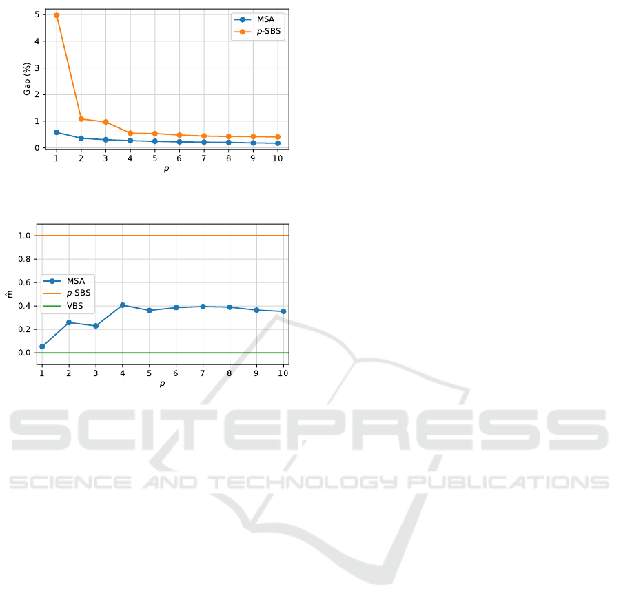
Figure 10: Gap percentage within the cost using p parame-

ter values and the best known cost, for MSA and p-SBS.

Figure 11: ˆm values for each p in the range [1, . . . , 10].

to test. For 4 or more parameter values, the difference

becomes minimal.

Another evaluation metric that is usually taken

into account for automatic algorithm selection tasks is

the ˆm metric, presented in Subsection 2.5. Figure 11

shows how the ˆm value behaves as p increases. We re-

call that values closer to 0 mean that the meta-solver

behaves close to the Virtual Best Solver and that val-

ues close to 1 mean that the solver behaves more like

the p-SBS. Note that while increasing p, the ˆm value

tends to get worse because the larger p is, the more

likely the performance of p-SBS is to improve.

5 CONCLUSIONS AND FUTURE

WORK

We demonstrate here that using ML for automatic

selection of an algorithm’s parameters improves sig-

niﬁcantly the quality of the solution provided. This

proof of concept is given here for the case of CVRP

and the sweep algorithm with the radius parameter.

We present a comparison of several ML algorithms

for selecting automatically the radius parameter. In

our experiments, KNN is the best performing. Using

KNN for automatically selecting the radius parame-

ter, we compare the performance of our meta-solver

(MSA) with two publicly available state-of-the-art

CVRP solvers: OR-tools (Perron and Furnon, 2019)

and FILO (Accorsi and Vigo, 2021) showing that au-

tomatic selection of the radius parameter provides fast

and high quality solutions. Speciﬁcally, MSA al-

ways dramatically improves on the quality and run-

ning time of OR-tools. For comparison with FILO

(which entails comparison with Clark-Wright), the

improvement is particularly notable for large-scale in-

stances with relatively small number of trucks (i.e. ra-

tio of total number of customers divided by the truck

capacity).

We further introduce here two new CVRP bench-

mark sets based on real addresses in Los Angeles and

New York City. These include about one million cus-

tomers each and a collection of 46000 instances that

are random subsets of these benchmarks.

Future research plans are to build a CVRP meta-

solver that considers a portfolio of additional algo-

rithms based on local search and exact methods. We

also plan to expand the functionality of the meta-

solver by adding capabilities of having user-speciﬁed

limits on the running time and other computational

resources.

ACKNOWLEDGEMENTS

This research was supported in part by AI Institute

NSF Award 2112533.

REFERENCES

Accorsi, L. and Vigo, D. (2021). A fast and scalable heuris-

tic for the solution of large-scale capacitated vehicle

routing problems. Transportation Science, 55(4):832–

856.

Agarap, A. F. (2018). Deep learning using rectiﬁed linear

units (relu). arXiv preprint arXiv:1803.08375.

Alesiani, F., Ermis, G., and Gkiotsalitis, K. (2022). Con-

strained clustering for the capacitated vehicle rout-

ing problem (cc-cvrp). Applied Artiﬁcial Intelligence,

pages 1–25.

Alloghani, M., Al-Jumeily, D., Mustaﬁna, J., Hussain, A.,

and Aljaaf, A. J. (2020). A systematic review on

supervised and unsupervised machine learning algo-

rithms for data science. Supervised and unsupervised

learning for data science, pages 3–21.

Alpaydin, E. (2021). Machine learning. MIT Press.

Applegate, D. L., Bixby, R. E., Chv

atal, V., Cook, W.,

Espinoza, D. G., Goycoolea, M., and Helsgaun, K.

(2009). Certiﬁcation of an optimal tsp tour through

85,900 cities. Operations Research Letters, 37(1):11–

15.

KDIR 2022 - 14th International Conference on Knowledge Discovery and Information Retrieval

Arnold, F., Gendreau, M., and S

orensen, K. (2019). Ef-

ﬁciently solving very large-scale routing problems.

Computers & operations research, 107:32–42.

Bogyrbayeva, A., Meraliyev, M., Mustakhov, T., and

Dauletbayev, B. (2022). Learning to solve vehi-

cle routing problems: A survey. arXiv preprint

arXiv:2205.02453.

Breiman, L. (1996). Bagging predictors. Machine learning,

24(2):123–140.

Breiman, L. (2001). Random forests. Machine learning,

45(1):5–32.

Burkart, N. and Huber, M. F. (2021). A survey on the ex-

plainability of supervised machine learning. Journal

of Artiﬁcial Intelligence Research, 70:245–317.

Carbone, R. and Armstrong, J. S. (1982). Note. evalua-

tion of extrapolative forecasting methods: results of a

survey of academicians and practitioners. Journal of

Forecasting, 1(2):215–217.

Clarke, G. and Wright, J. W. (1964). Scheduling of vehicles

from a central depot to a number of delivery points.

Operations research, 12(4):568–581.

Dondo, R. and Cerd

a, J. (2013). A sweep-heuristic based

formulation for the vehicle routing problem with

cross-docking. Computers & Chemical Engineering,

48:293–311.

Dunning, I., Gupta, S., and Silberholz, J. (2018). What

works best when? a systematic evaluation of heuris-

tics for max-cut and qubo. INFORMS Journal on

Computing, 30(3):608–624.

Elshaer, R. and Awad, H. (2020). A taxonomic review of

metaheuristic algorithms for solving the vehicle rout-

ing problem and its variants. Computers & Industrial

Engineering, 140:106242.

Fellers, J., Quevedo, J., Abdelatti, M., Steinhaus, M., and

Sodhi, M. (2021). Selecting between evolutionary and

classical algorithms for the cvrp using machine learn-

ing: optimization of vehicle routing problems. In Pro-

ceedings of the Genetic and Evolutionary Computa-

tion Conference Companion, pages 127–128.

Fix, E. and Hodges, J. L. (1989). Discriminatory analy-

sis. nonparametric discrimination: Consistency prop-

erties. International Statistical Review/Revue Interna-

tionale de Statistique, 57(3):238–247.

Friedman, J. H. (2001). Greedy function approximation: a

gradient boosting machine. Annals of statistics, pages

1189–1232.

Fukushima, K. and Miyake, S. (1982). Neocognitron: A

self-organizing neural network model for a mecha-

nism of visual pattern recognition. In Competition and

cooperation in neural nets, pages 267–285. Springer.

Gillett, B. E. and Miller, L. R. (1974). A heuristic algo-

rithm for the vehicle-dispatch problem. Operations

research, 22(2):340–349.

Haimovich, M. and Rinnooy Kan, A. H. (1985). Bounds

and heuristics for capacitated routing problems. Math-

ematics of operations Research, 10(4):527–542.

Huerta, I. I., Neira, D. A., Ortega, D. A., Varas, V., Godoy,

J., and As

ın-Ach

a, R. (2022). Improving the state-of-

the-art in the traveling salesman problem: An anytime

automatic algorithm selection. Expert Systems with

Applications, 187:115948.

Kerschke, P., Hoos, H. H., Neumann, F., and Trautmann, H.

(2019). Automated algorithm selection: Survey and

perspectives. Evolutionary computation, 27(1):3–45.

Lin, S. and Kernighan, B. W. (1973). An effective heuristic

algorithm for the traveling-salesman problem. Opera-

tions research, 21(2):498–516.

Lindauer, M., Hoos, H. H., Hutter, F., and Schaub, T.

(2015). Autofolio: An automatically conﬁgured al-

gorithm selector. Journal of Artiﬁcial Intelligence Re-

search, 53:745–778.

Lindauer, M., van Rijn, J. N., and Kotthoff, L. (2019). The

algorithm selection competitions 2015 and 2017. Ar-

tiﬁcial Intelligence, 272:86–100.

opez-Ib

nez, M., Dubois-Lacoste, J., C

aceres, L. P., Bi-

rattari, M., and St

utzle, T. (2016). The irace package:

Iterated racing for automatic algorithm conﬁguration.

Operations Research Perspectives, 3:43–58.

McCulloch, W. S. and Pitts, W. (1943). A logical calculus

of the ideas immanent in nervous activity. The bulletin

of mathematical biophysics, 5(4):115–133.

Perron, L. and Furnon, V. (2019). Or-tools.

Pessoa, A. A., Poss, M., Sadykov, R., and Vanderbeck, F.

(2021). Branch-cut-and-price for the robust capac-

itated vehicle routing problem with knapsack uncer-

tainty. Operations Research, 69(3):739–754.

Quinlan, J. R. (1986). Induction of decision trees. Machine

learning, 1(1):81–106.

Rice, J. R. (1976). The algorithm selection problem. In Ad-

vances in computers, volume 15, pages 65–118. Else-

vier.

Schapire, R. E. (1997). Using output codes to boost multi-

class learning problems. In ICML, volume 97, pages

313–321. Citeseer.

Schapire, R. E. (2013). Explaining adaboost. In Empirical

inference, pages 37–52. Springer.

Stone, M. (1974). Cross-validatory choice and assessment

of statistical predictions. Journal of the royal statis-

tical society: Series B (Methodological), 36(2):111–

133.

Zhu, X. and Goldberg, A. B. (2009). Introduction to semi-

supervised learning. Synthesis lectures on artiﬁcial

intelligence and machine learning, 3(1):1–130.

Fast Algorithms for the Capacitated Vehicle Routing Problem using Machine Learning Selection of Algorithm’s Parameters