A Suite of Incremental Image Degradation Operators for Testing Image

Classiﬁcation Algorithms

Kevin Swingler

Computing Sciene and Mathematics, University of Stirling, Stirling, FK9 4LA, U.K.

Keywords:

Adversarial Images, Model Robustness, Degraded Image Performance.

Abstract:

Convolutional Neural Networks (CNN) are extremely popular for modelling sound and images, but they suffer

from a lack of robustness that could threaten their usefulness in applications where reliability is important.

Recent studies have shown how it is possible to maliciously create adversarial images—those that appear to

the human observer as perfect examples of one class but that fool a CNN into assigning them to a different,

incorrect class. It takes some effort to make these images as they need to be designed speciﬁcally to fool a

given network. In this paper we show that images can be degraded in a number of simple ways that do not need

careful design and that would not affect the ability of a human observer, but which cause severe deterioration

in the performance of three different CNN models. We call the speed of the deterioration in performance due

to incremental degradations in image quality the degradation proﬁle of a model and argue that reporting the

degradation proﬁle is as important as reporting performance on clean images.

1 INTRODUCTION

Convolutional Neural Networks (CNNs) are increas-

ingly criticised for being fragile, meaning that they

fail on inputs that are out of the distribution (OOD)

of the training data or on inputs that are deliberately

altered to cause failure (Heaven, 2019). Such in-

puts are often known as adversarial inputs. This pa-

per proposes a methodology for testing the robust-

ness of CNN models for computer vision, showing

how the degradation proﬁle of a model can be used

to measure robustness and compare one model with

another. Some simple image degradation operators,

which would not fool a human viewer are shown to

signiﬁcantly reduce model accuracy. The operators

are incremental, in the sense that repeated application

causes increased degradation, and we ﬁnd that model

accuracy falls as the level of degradation increases.

What’s more, the ranking of the correct label in the list

of model outputs drops as an image degrades, as does

the probability assigned to the correct label. We call

these three measures the accuracy degradation pro-

ﬁle, the rank degradation proﬁle and the probability

degradation proﬁle. These measures degrade faster

for less robust models.

Three different models are compared: ResNet50

(He et al., 2016), the B0 version of EfﬁcientNet (Tan

https://orcid.org/0000-0002-4517-9433

and Le, 2019), and version 3 of the Inception model

(Szegedy et al., 2016). The implementations readily

available in Keras were utilised, using the standard

weights from the Imagenet training data. No addi-

tional training was performed. These models were

chosen because they are widely accessible and widely

used, so their robustness is of interest. The paper is

not designed as a ranking of these algorithms—they

are chosen as illustrations only.

1.1 Background and Motivation

CNNs have become the state-of-the-art in computer

vision over the past decade, performing at or even

in excess of human levels of accuracy (Chen et al.,

2015). They have found application in industry, se-

curity, entertainment and medicine and will play a

crucial role in advances in technology such as self-

driving cars. It is becoming increasingly clear, how-

ever, that current CNN models are not as robust as

they need to be (Heaven, 2019), and if they are to be

relied on to drive us safely home or detect cancer in

a scan, then we need to be able to trust them not to

make mistakes (Maron et al., 2021a), (Maron et al.,

2021b), (Finlayson et al., 2019).

There are a small number of standard measures

of model quality. Most papers report accuracy (the

percentage of correctly classiﬁed images) and other

262

Swingler, K.

A Suite of Incremental Image Degradation Operators for Testing Image Classiﬁcation Algorithms.

DOI: 10.5220/0011511000003332

In Proceedings of the 14th International Joint Conference on Computational Intelligence (IJCCI 2022), pages 262-272

ISBN: 978-989-758-611-8; ISSN: 2184-3236

derived measures such as precision, recall or f-score.

These measures are calculated from a dataset that is

removed from the training corpus before the mod-

elling process begins so they are independent of that

process. They are, however, generally taken from the

same distribution as the training data. Recently, there

has been an increased amount of work addressing the

question of performance on out of distribution (OOD)

examples. These are images that clearly belong to one

of the target classes for the model, but which have

been altered in some way to make them novel to the

classiﬁer.

Much of the recent work in this ﬁeld has concen-

trated on adversarial images, which are images that

are generated with the intention of fooling a classi-

ﬁer, often guided by the classiﬁer itself. In an early

example of this (Szegedy et al., 2013) used the gra-

dients at the output layer of a classiﬁcation CNN to

guide small changes to the input pixels that would

leave the input image visually unchanged but elicit an

incorrect classiﬁcation from the model. Other simi-

lar results have followed, while others have taken the

opposite view and produced images that are classi-

ﬁed with high conﬁdence by a CNN but which are

completely unrecognisable to humans (Nguyen et al.,

2015). Other approaches use rendering software to

produce images in which the object to be classiﬁed is

in an unusual pose (Alcorn et al., 2019) or to ﬁlter im-

ages to ﬁnd those that are naturally difﬁcult for CNNs

to classify (Hendrycks et al., 2019).

Some methods follow the gradients of the model

and some make use of gradient free optimisation tech-

niques (Uesato et al., 2018). Others make use of ad-

versarial images generated using a surrogate model

that was trained on a similar (or the same) data set.

These are known as transfer based attacks (Papernot

et al., 2017). Methods that make use of the gradients

accessible in an image may be classed as white box

attacks, as they are guided by access to the model.

Other adversarial methods, known as black box at-

tacks, degrade input images in a way that would not

cause a human observer any difﬁculty in making a

classiﬁcation, but which can fool a CNN model. For

example, (Engstrom et al., 2019) explore the effects

of rotations and translations on classiﬁer robustness.

They also point out that there is a focus in the liter-

ature on ﬁnding small image perturbations (in some

p-norm measure) but that humans might classify two

images as being of the same class even if there are

large differences in the pixel values.

Not all adversarial attacks involve manipulating

an existing image. A number of researchers have pro-

duced stickers that can be used to defeat computer vi-

sion algorithms by placing them in a real world scene.

For example, (Komkov and Petiushko, 2021) show

how stickers worn on a hat confuse the state-of-the-art

ArcFace face recognition model. (Thys et al., 2019)

developed a patch that can be printed and held by a

person, which is capable of hiding them from a per-

son detection algorithm.

We make the distinction between targeted adver-

sarial examples and degraded examples. The assump-

tion in a lot of the work on adversarial images is that

a malicious agent generates images to fool a CNN

classiﬁer. The assumption behind degraded images in

more benign: simply that variations in light, weather,

image quality, occlusion and color occur naturally and

may impact the performance of classiﬁers. Of course,

images may also be degraded by malicious agents and

some of the degradations proposed in this paper are

both effective and trivial to apply.

We conclude that CNNs are not as robust as they

need to be, that they are easily fooled into making

errors and that a measure of robustness would be an

important step towards addressing that issue. The rest

of the paper proposes a series of such measures and

illustrates their use on three popular CNN models.

1.2 Degradation Operators

Fourteen degradation operators were tested, each with

30 different levels of degradation from the original

image. All the operators have the quality that each

subsequent level of degradation increases the differ-

ence from the original image. Operators can be char-

acterised as either global, where every pixel in the im-

age is altered at each level, or local, where only some

pixels are altered. They may also be characterised as

being deterministic, where the same degradation has

the same effect in repeated applications to the same

image, or stochastic, where the effect of applying

a degradation is drawn at random from some distri-

bution. Operators may also be either colour based,

where the colour palette is altered, or pixel based,

where the alterations are to individual pixels.

Each level of a degradation has a degree to which

it is applied. For example, if random pixel values are

changed, the degree is the number of pixels altered

at a single level. These degree parameters are chosen

experimentally to produce a degradation to near zero

accuracy after 30 levels.

The following sections brieﬂy describe and char-

acterise each degradation operator. Unless stated oth-

erwise, the phrase randomly selected means that sam-

ples were drawn from a uniform distribution.

Random Lines. Lines of one pixel width are drawn

onto the image with anti-aliasing. Lines start at a ran-

A Suite of Incremental Image Degradation Operators for Testing Image Classiﬁcation Algorithms

263

dom location on the left or top edge of the image and

end at a random location on the right or bottom edge,

meaning they have a location and orientation both

drawn from a uniform random distribution. Two dif-

ferent operators are deﬁned, one which draws white

lines and one which draws black lines. This operator

is local, stochastic and pixel based. A single line is

added at each level of the degradation.

Random Boxes. Small black rectangles are drawn

onto the image, with random locations and with

height and width chosen from a uniform random dis-

tribution over 2 to 5 pixels. This operator is local,

stochastic and pixel based. The number of rectangles

added at each level of the degradation is (h + w)/10

where h and w are the height and width of the image

respectively.

Global Blur. A ﬁve by ﬁve pixel uniform blur is ap-

plied to the image by replacing each color channel

value for each pixel by the average of the values in

a 5 × 5 square neighbourhood around the pixel. Re-

peated application of the operator leads to increased

levels of blur. This operator is global, deterministic

and pixel based.

Local Blur. Small rectangular areas of the image

are replaced by the average value of the pixels in that

rectangle (for each color channel). Rectangle loca-

tions are selected at random from a uniform distribu-

tion over the image and height and width are selected

uniformly at random from [2, 10] pixels. This opera-

tor is local, stochastic and pixel based. The number

of rectangles added at each level of the degradation is

(h + w).

Random Noise. A number of pixels, chosen at ran-

dom, have their colours changed to a new, random

color. This operator is local, stochastic and pixel

based. The number of pixels changed at each itera-

tion is wh/50.

Random Pixel Exchange. Pairs of pixel locations

are selected at random and the color values of the

two locations are exchanged, so that the pixels ef-

fectively swap locations. The number of pixels ex-

changed at each iteration is wh/20. This operator is

local, stochastic and pixel based.

Random Adjacent Pixel Exchange. Pairs of adja-

cent pixels are swapped. The location of the ﬁrst pixel

is chosen at random and the location of the second is

chosen at random from the eight adjacent locations

around the ﬁrst. The number of pixels exchanged

at each iteration is wh/20. This operator is local,

stochastic and pixel based.

White Fog. Pixel locations are selected at random

and the color of the chosen pixels is faded towards

white. The fading is done by adding 20 to each of

the colour channels and clipping each at 255. The

number of pixels exchanged at each iteration is wh/5.

This operator is local, stochastic and pixel based.

Fade to Black, White or Greyscale. The whole

image has its color space altered so that it fades to-

wards a chosen target palette, either an all black im-

age, an all white image, or the image in greyscale.

To fade towards black, each color channel of each

pixel is multiplied by 0.9 and to fade to white, they

are multiplied by 1.1. The move towards greyscale is

achieved by converting the image to the HSV colour

space, multiplying the saturation channel by 0.9, and

then converting back to the RGB colour space. These

operators are global, deterministic and color based.

Posterize. The number of colors in the palette of the

image is reduced at each iteration. A simple method is

used, in which each color channel is discretized sep-

arately into a chosen number of distinct values. The

color range from 0 to 255 is split into b bins, each of

size 255/b. The color value for bin i is calculated as

(i + 1)255/b. The bin count, b starts at 32 in these

experiments and decreases by one each iteration until

it reaches 2 at the last level. This operator is global,

deterministic and color based.

JPEG Compress. Images are compressed using

JPEG compression with increasingly high levels of

compression. In this work, the imencode() func-

tion of the Python OpenCV library was used to en-

code each image, which was then reconstructed using

imdecode() to produce a degraded image. The degree

of compression over 30 iterations started at 32 and ﬁn-

ished at 2. This operator is global, deterministic and

color based.

Model Gradient Descent. This is the only one of

the degradation operators that relies on access to the

model being used to make the classiﬁcations. It fol-

lows (Szegedy et al., 2013) by following the gradients

of the output probabilities from the model, back prop-

agating them to the input layer to make small changes

to the input image that move the classiﬁcation away

from the correct output. This operator is local, deter-

ministic and pixel based.

NCTA 2022 - 14th International Conference on Neural Computation Theory and Applications

264

1.3 Approximating Real World

Degradation

All but one of the operators described above are ap-

plied without knowledge of the model that will be

used to make classiﬁcations. They can all be applied

very simply to source images in digital form. Some

may also be applied to real world scenes before the

scene is photographed and some are approximations

to real world degradations in image quality. Placing

small black or white rectangular stickers onto objects

such as road signs has been shown to confuse classi-

ﬁcation models (Eykholt et al., 2018) and we approx-

imate that with the Random Boxes operator. Simi-

larly, it would be possible to draw thin black lines

across objects that you did not want detected. The

Local Blur operator is an approximation to the effects

of grease or water on a lens, blurring small areas of

the image. The Fade to Black operator approximates

darkness and the fade to white operator approximates

saturation due to bright light. Both situations occur

naturally in vehicle driving situations. The White Fog

operator approximates the effects of fog or smoke in

a scene and and the Posterise and JPEG Compression

operators investigate the effects of poor quality sen-

sors or storage compression. We include one adver-

sarial example—the Gradient Descent—for compar-

ison, but this paper is primarily concerned with de-

graded images rather than carefully designed attacks.

2 METHODOLOGY

The degradation proﬁle for three popular CNN image

classiﬁcation algorithms was calculated. The models

are the 50 layer version of ResNet (ResNet50) (He

et al., 2016), the B0 version of EfﬁcientNet (Efﬁcient-

NetB0) (Tan and Le, 2019), and version 3 of the In-

ception model (InceptionV3) (Szegedy et al., 2016),

all using the default weights trained on the Imagenet

dataset. The Keras implementation of these models

was used. Models were tested using a small sample

of 590 images from the Imagenet training set, all se-

lected for being correctly classiﬁed by the ResNet50

model. Three measures of performance were calcu-

lated: Accuracy is the proportion of correctly classi-

ﬁed images over the dataset. Label Rank is the av-

erage index position of the correct label in the model

output list, sorted by probability. A score of 5 sug-

gests that the model is often incorrect, but that the

correct answer is still in the top ﬁve. There are 1000

class labels in the Imagenet dataset so a model that is

no better than chance would score around 500. Label

Probability is the average probability assigned by the

model to the output label that is known to be correct.

The models have a softmax at the output layer, so we

expect the probability assigned to non-winning labels

to be low.

For each model, the testing regime was as follows:

For each degradation operator, all 590 images are pre-

sented to the model once for each of the 30 levels of

degradation. The three performance measures were

recorded for each level. The images are of different

sizes, but the models expect an input of a ﬁxed size,

so the images were resized before the degradation op-

erations were applied, meaning that the pixel based

operations really did alter single pixels in the images

processed by the models. That is to say that the degra-

dations were not subject to scaling.

3 RESULTS

Over three models, fourteen degradation operators, 30

levels of degradation, and three performance metrics,

there are many ways to analyse the results. The sim-

plest aggregation is to calculate the average of each

performance metric for each model. This gives an

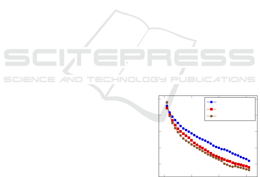
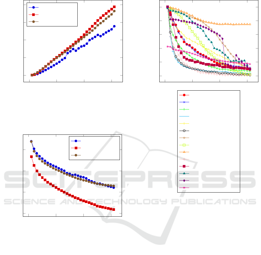
easily digested comparison among the models. Fig-

ures 1, 2 and 3 show the average of the three perfor-

mance metrics: accuracy, ranks and probability, by

level, for each of the three models. They show that

InceptionV3 is the most robust across all three mea-

sures. Note that for the correct label rank measure,

low values are closer to the top, so the winning label

has a rank of zero.

0 10 20 30

0.2

0.4

0.6

0.8

Degradation level

Accuracy

InceptionV3

EfﬁcientNetB0

ResNet50

Figure 1: The accuracy degradation proﬁle for ResNet50,

EfﬁcientNetB0 and InceptionV3 across 30 levels of input

image degradation. The average is taken over 14 different

degradation operators.

A Suite of Incremental Image Degradation Operators for Testing Image Classiﬁcation Algorithms

265

0 10 20 30

100

150

200

Degradation level

Average Rank of Correct Label

InceptionV3

EfﬁcientNetB0

ResNet50

Figure 2: The rank degradation proﬁle for ResNet50, Efﬁ-

cientNetB0 and InceptionV3 across 30 levels of input image

degradation. The average is taken over 14 different degra-

dation operators.

0 10 20 30

0.2

0.4

0.6

0.8

Degradation level

Average Probability of Correct Label

InceptionV3

EfﬁcientNetB0

ResNet50

Figure 3: The probability degradation proﬁle for ResNet50,

EfﬁcientNetB0 and InceptionV3 across 30 levels of input

image degradation. The average is taken over 14 different

degradation operators.

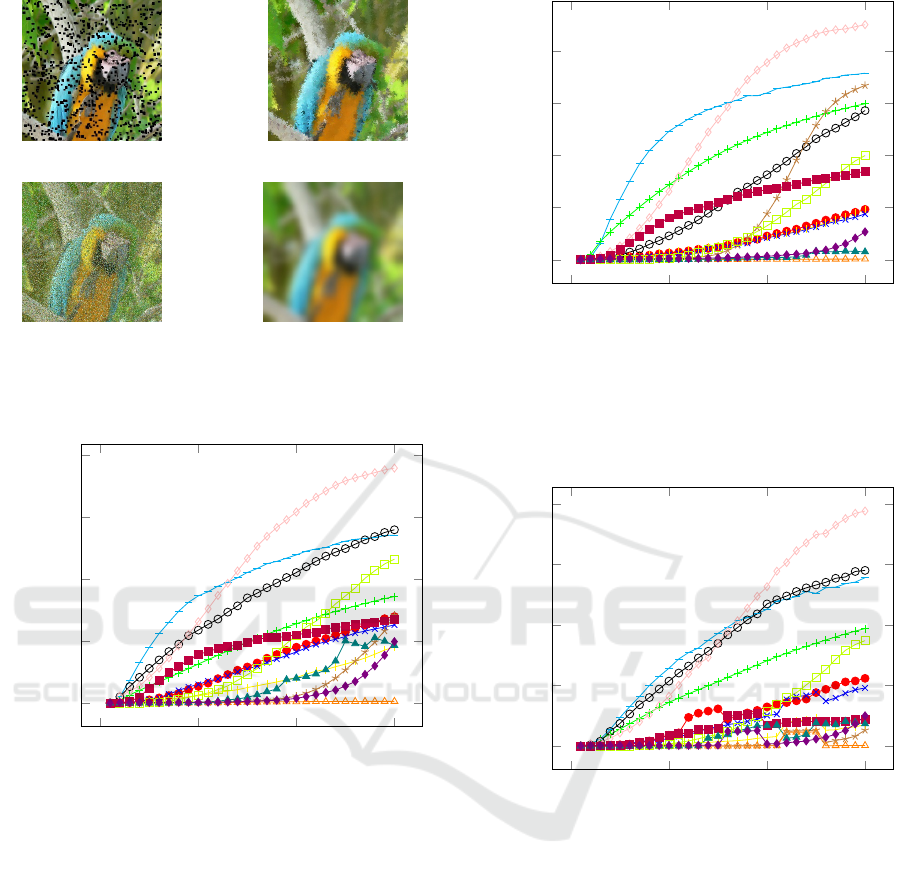
3.0.1 Degradation Proﬁle by Model

The degradation proﬁle of a model, given a test set

and a degradation operator describes the performance

of the model on increasingly degraded versions of the

images in a data set for which it was originally ca-

pable of achieving 100% classiﬁcation accuracy. The

steeper the curve, the more fragile the model is judged

to be. We compare the proﬁle of each operator in

turn. Figures 4, 5, and 6 show the proﬁles for ResNet

50, EfﬁcientNet B0 and Inception V3. Looking at

these ﬁgures, we learn that all networks are robust to

changes from full colour to grey scale and all are par-

ticularly vulnerable to blurring an image or swapping

the values in a few pixel pairs.

0 10 20 30

0.2

0.4

0.6

0.8

Degradation level

Accuracy

Black lines

White lines

Global Blur

Rand adj pixel swap

White fog

Random Boxes

Fade black

Fade white

Fade grey

Swap rand pixels

Local blur

Posterise

JPEG

Gradient Descent

Figure 4: The accuracy degradation proﬁle for ResNet50

for 14 different degradation operators. The y axis shows ac-

curacy and the x axis increases with the degree of degrada-

tion. The model is particularly vulnerable to the addition of

small black rectangles, the swapping of pixel locations and

blurring of the image. It can also be quickly fooled using

gradient descent away from the winning category.

3.1 Example Failure Points

In this section we investigate the degree to which an

image needs to be degraded before the average accu-

racy of a CNN classiﬁer drops below 50% on the test

data. Tables 1, 2, and 3 describe the degree of degra-

dation required to move each of the three models from

100% accuracy to 50% accuracy. The percentage of

the pixels in the original image that are changed as a

result of each degradation is given, along with a de-

scription of the change. This measure is only mean-

ingful for the pixel based operators, as the global op-

erators alter every pixel in an image. The three op-

erators that require the fewest pixels to change be-

fore accuracy drops below 50% are those that draw

lines or small boxes onto the image. In the case of

the small boxes, for example, only 3% of the pixels

need to be changed in the images in the test set be-

NCTA 2022 - 14th International Conference on Neural Computation Theory and Applications

266

0 10 20 30

0.2

0.4

0.6

0.8

Degradation level

Accuracy

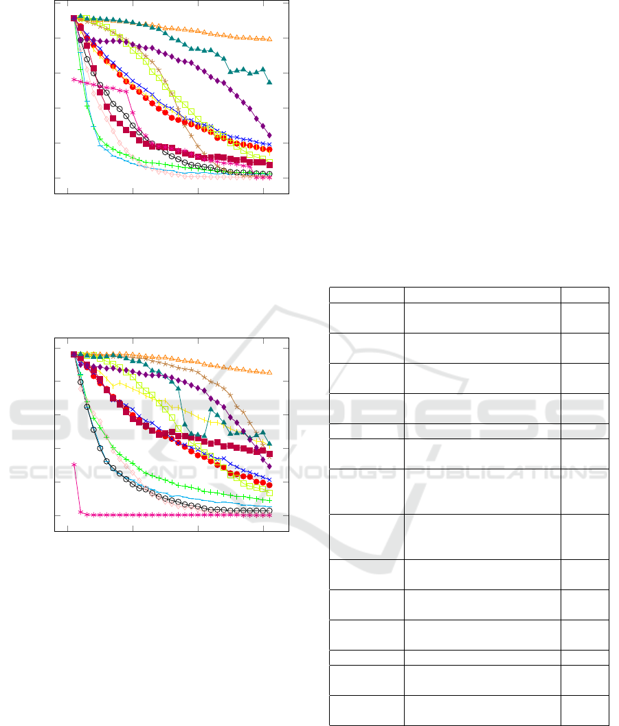
Figure 5: The accuracy degradation proﬁle for EfﬁcientNet

B0 for 14 different degradation operators. The y axis shows

accuracy and the x axis increases with the degree of degra-

dation. The model is particularly vulnerable to the swap-

ping of pixel locations and blurring of the image. Refer to

ﬁgure 4 for the legend.

0 10 20 30

0.2

0.4

0.6

0.8

Degradation level

Accuracy

Figure 6: The accuracy degradation proﬁle for Inception

V3 for 14 different degradation operators. The y axis shows

accuracy and the x axis increases with the degree of degra-

dation. The model is particularly vulnerable to the addition

of small black rectangles, the swapping of pixel locations

and blurring of the image. Refer to ﬁgure 4 for the legend.

fore the accuracy drops below 50% for the ResNet50

model. The degradations that the models are most ro-

bust to are the color saturation based operators: fade

to black, fade to white and fade to grey scale. All

three models are very robust under a change from full

color to grey scale, maintaining around 80% accuracy

even when the image is reduced completely to grey

scale. Similarly, the models are robust to a reduction

in the number of colours in the palette. EfﬁcientNet is

particularly robust, achieving 55% accuracy when the

palette is reduced to just 8 colors.

The gradient descent operator is the only one we

employ that is aided by access to the model itself. By

following the steepest gradient away from the win-

ning category label, an adversarial image is generated,

which is similar to the original image, but produces a

different output label. A more robust model will re-

quire a greater number of steps down the classiﬁcation

gradient before the output class is changed. Of the

three models we investigate here, ResNet50 and Efﬁ-

cientNetB0 are far more brittle than the Inception V3

model, with the number of steps required to change

the labels on 50% of the test set being 1, 4 and 22 for

the models respectively.

Table 1: The average change made to images in the test set

to reduce the accuracy of the ResNet50 model from 100%

to 50% on that dataset. The % Ch. column contains the

number of pixels changed as a percentage of those in the

image.

Degr. Change Made Ch.

Black

Lines

6 randomly placed 1 pixel

wide lines

White

Lines

7 randomly placed 1 pixel

wide lines

Random

Boxes

90 boxes 3%

Global

blur

4 consecutive 5×5 convo-

lutions

100%

Local blur 1792 local blur boxes 70%

Noise 8% of pixels replaced

with a random color

Swap Ad-

jacent Pix-

els

56% of pixels changed 56%

Swap

Rand.

Pixels

9% of pixels changed 9%

White Fog Average pixel values in-

creased: 151 to 187

86%

Fade

Black

Average pixel values re-

duced: 151 to 18

100%

Fade

White

Average pixel values in-

creased: 151 to 250

100%

Posterise Reduced to 151 Colors 100%

JPEG

Compress

Reduced to 135 Colors 100%

Gradient

Descent

1 Iteration 100%

3.2 Visualising the Effects of

Degradation

To help the reader visualise the degree to which im-

ages need to be changed to produce a signiﬁcant drop

in model performance, we present some visual exam-

A Suite of Incremental Image Degradation Operators for Testing Image Classiﬁcation Algorithms

267

Table 2: The average change made to images in the test set

to reduce the accuracy of the EfﬁcientNetB0 model from

100% to 50% on that dataset. The % Ch. column contains

the number of pixels changed as a percentage of those in the

image.

Degr. Change Made Ch.

Black

Lines

10 randomly placed 1

pixel wide lines

10%

White

Lines

12 randomly placed 1

pixel wide lines

13%

Random

Boxes

224 boxes 8%

Global

blur

2 consecutive 5×5 convo-

lutions

100%

Local blur 896 local blur boxes 70%

Noise 16% of pixels replaced

with a random color

16%

Swap Ad-

jacent Pix-

els

56% of pixels changed 56%

Swap

Random

Pixels

13% of pixels changed 13%

White Fog Average pixel values in-

creased: 151 to 190

89%

Fade

Black

Average pixel values re-

duced: 151 to 31

100%

Fade

White

Average pixel values in-

creased: 151 to 253

100%

Posterise Reduced to 8 Colors 100%

JPEG

Compress

Reduced to 25 Colors 100%

Gradient

Descent

5 Iterations 100%

ples. Speciﬁcally, we present examples of images that

move an Inception V3 model from 100% accuracy to

90%, 50% and 10% respectively. For each degrada-

tion operator, the accuracy proﬁle is used to ﬁnd the

number of times the degradation needs to be applied

to ﬁrst cause the accuracy to drop below the target

threshold on the test dataset. A single example im-

age is then degraded this many times to produce an

example image. These images are just examples, but

they illustrate to the human viewer how little or much

degradation is needed to cause a drop in performance

from slight to catastrophic.

4 OTHER MEASURES OF

ROBUSTNESS

CNN models have an output layer that associates a

score or probability with every possible class label.

Classiﬁcation is performed by identifying the label

Table 3: The average change made to images in the test

set to reduce the accuracy of the Inception V3 model from

100% to 50% on that dataset. The % Ch. column contains

the percentage of pixels changed in the image.

Degr. Change Made Ch.

Black

Lines

13 randomly placed 1

pixel wide lines

14%

White

Lines

14 randomly placed 1

pixel wide lines

13%

Random

Boxes

176 boxes 7%

Global

blur

5 consecutive 5×5 convo-

lutions

100%

Local blur 5824 local blur boxes 77%

Noise 24% of pixels replaced

with a random color

24%

Swap Ad-

jacent Pix-

els

78% of pixels changed 78%

Swap

Random

Pixels

22% of pixels changed 22%

White Fog Average pixel values in-

creased: 151 to 225

100%

Fade

Black

Average pixel values re-

duced: 151 to 8

100%

Fade

White

Average pixel values in-

creased: 151 to 253

100%

Posterise 85 Colors 100%

JPEG

Compress

Reduced to 23 Colors 100%

Gradient

Descent

Reduced to 22 Iterations 100%

with the highest score. A model might be considered

more robust if a degradation causes the correct label

to be rated as the second most probable rather than

the 10th. Where the probabilities of the top rated cat-

egories are close, there are methods based on context

(Chu and Cai, 2018) that might help disambiguate the

confusion. Therefore, it is useful to know the proba-

bility assigned to the correct label and how far down

the probability rankings a degradation moves the cor-

rect label. We measure the average probability and

the average rank of the correct class across our test

dataset for each degree of degradation. We call these

the probability degradation proﬁle and the rank degra-

dation proﬁle.

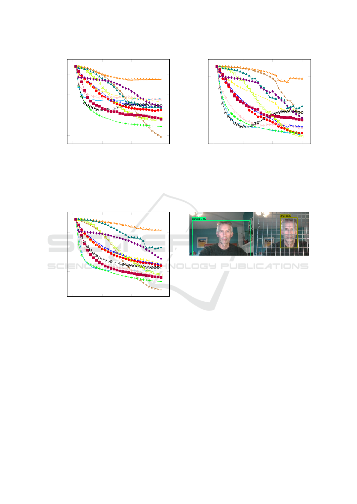
Figures 10, 11 and 12 show the rank degrada-

tion proﬁles for ResNet50, EfﬁcientNetB0 and Incep-

tion V3, respectively and ﬁgures 13, 14 and 15 show

the probabiliy degradation proﬁles for ResNet50, Ef-

ﬁcientNetB0 and Inception V3, respectively.

NCTA 2022 - 14th International Conference on Neural Computation Theory and Applications

268

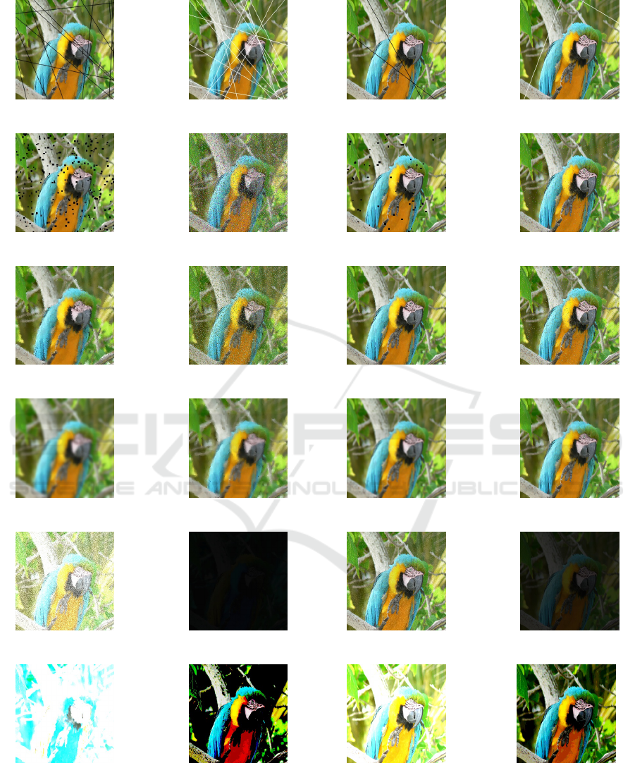
(a) Black lines. (b) White Lines.

(e) Adj. Pixel Swap. (f) Rand. Pixel Swap.

(g) Global Blur. (h) Local Blur.

(i) White Fog. (j) Fade to Black.

(k) Fade to white. (l) Posterise.

Figure 7: Example degraded images at the ﬁrst point where

the accuracy measure for our test data ﬁrst drops from 100%

to below 50%.

(a) Black lines. (b) White Lines.

(e) Adj. Pixel Swap. (f) Rand. Pixel Swap.

(g) Global Blur. (h) Local Blur.

(i) White Fog. (j) Fade to Black.

(k) Fade to white. (l) Posterise.

Figure 8: Example degraded images at the ﬁrst point where

the accuracy measure for our test data ﬁrst drops from 100%

to below 90%.

A Suite of Incremental Image Degradation Operators for Testing Image Classiﬁcation Algorithms

269

(a) Small Boxes. (b) Adj. Pixel Swap.

Figure 9: Example degraded images at the ﬁrst point where

the accuracy measure for our test data ﬁrst drops from 100%

to below 10%.

0 10 20 30

100

200

300

400

Degradation level

Accuracy

Figure 10: The rank degradation proﬁle for ResNet50 for

14 different degradation operators. The y axis shows aver-

age ranking of the correct label and the x axis increases with

the degree of degradation. The three most damaging degra-

dations are swapping pixel pairs, and occluding with small

rectangles. Refer to ﬁgure 4 for the legend.

5 CONCLUSIONS AND FURTHER

WORK

It is clear that some of the commonly used computer

vision CNN models are easily fooled by a range of

image degradations. By presenting a suite of sim-

ple degradation operators, we hope to encourage re-

searchers to include a measure of robustness in ad-

dition to accuracy measures when presenting new

algorithms or architectures. We found that three

commonly used CNN architectures were robust to

changes in the color palette, but that small pixel

0 10 20 30

100

200

300

400

Degradation level

Accuracy

Figure 11: The rank degradation proﬁle for EfﬁcientNet B0

for 14 different degradation operators. The y axis shows

average ranking of the correct label and the x axis increases

with the degree of degradation. The three most damaging

degradations are swapping pixel pairs, and occluding with

small rectangles. Refer to ﬁgure 4 for the legend.

0 10 20 30

100

200

300

400

Degradation level

Accuracy

Figure 12: The rank degradation proﬁle for Inception V3

for 14 different degradation operators. The y axis shows

average ranking of the correct label and the x axis increases

with the degree of degradation. The three most damaging

degradations are swapping pixel pairs, and occluding with

small rectangles. Refer to ﬁgure 4 for the legend.

level changes such as drawing thin lines or swap-

ping random pixel values cause severe degradation

in accuracy. We show some examples where the ac-

curacy of the CNN falls below 10%, and the iden-

tity of the object is still clear to the human eye.

We hope that more researchers will include mea-

sures of robustness when they report the performance

of new computer vision algorithms. To this end,

the code to perform the image degradations and as-

sociated experiments may be found on github at

https://github.com/kevswingler/ImageDegrade.

NCTA 2022 - 14th International Conference on Neural Computation Theory and Applications

270

0 10 20 30

0.2

0.4

0.6

0.8

Degradation level

Accuracy

Figure 13: The probability degradation proﬁle for ResNet50

for 14 different degradation operators. The y axis shows the

average probability assigned to the correct label and the x

axis increases with the degree of degradation. The three

most damaging degradations are swapping pixel pairs, and

occluding with small rectangles. Refer to ﬁgure 4 for the

legend.

0 10 20 30

0.2

0.4

0.6

0.8

Degradation level

Accuracy

Figure 14: The probability degradation proﬁle for Efﬁcient-

Net B0 for 14 different degradation operators. The y axis

shows the average probability assigned to the correct label

and the x axis increases with the degree of degradation. The

three most damaging degradations are swapping pixel pairs,

and occluding with small rectangles. Refer to ﬁgure 4 for

the legend.

We are curious to see whether the simple degrada-

tions we propose can be used live. For example, rather

than use a carefully designed patch to fool a person

detector, as proposed by (Thys et al., 2019), simple

props are often sufﬁcient. The question of computer

vision camouﬂage is the subject of ongoing work, but

ﬁgure 16 shows one small example where an SSD

MobileNet object detection algorithm trained on the

MS-COCO dataset is fooled into labelling a person as

a dog with the aid of nothing more sophisticated than

0 10 20 30

0.4

0.6

0.8

Degradation level

Accuracy

Figure 15: The probability degradation proﬁle for Inception

V3 for 14 different degradation operators. The y axis shows

the average probability assigned to the correct label and the

x axis increases with the degree of degradation. The three

most damaging degradations are swapping pixel pairs, and

occluding with small rectangles. Refer to ﬁgure 4 for the

legend.

Figure 16: It is easy to fool an SSD object detector by sim-

ply holding a grid in front of yourself - here the classiﬁca-

tion changes from person to dog.

a cake cooling rack.

As the robustness of models improves, the type

of degradations that should be tested will evolve and

we do not expect the operations described here to be

challenging for long. We hope that other authors will

propose further tests and that some kind of arms race

will enhance the robustness of all models. We hope,

of course, that the algorithm developers win the race

but at the moment what is important is that they start

to take part.

REFERENCES

Alcorn, M. A., Li, Q., Gong, Z., Wang, C., Mai, L., Ku, W.-

S., and Nguyen, A. (2019). Strike (with) a pose: Neu-

ral networks are easily fooled by strange poses of fa-

miliar objects. In Proceedings of the IEEE/CVF Con-

ference on Computer Vision and Pattern Recognition,

pages 4845–4854.

Chen, L., Wang, S., Fan, W., Sun, J., and Naoi, S.

(2015). Beyond human recognition: A cnn-based

A Suite of Incremental Image Degradation Operators for Testing Image Classiﬁcation Algorithms

271

framework for handwritten character recognition. In

2015 3rd IAPR Asian Conference on Pattern Recogni-

tion (ACPR), pages 695–699. IEEE.

Chu, W. and Cai, D. (2018). Deep feature based con-

textual model for object detection. Neurocomputing,

275:1035–1042.

Engstrom, L., Tran, B., Tsipras, D., Schmidt, L., and

Madry, A. (2019). Exploring the landscape of spatial

robustness. In International Conference on Machine

Learning, pages 1802–1811. PMLR.

Eykholt, K., Evtimov, I., Fernandes, E., Li, B., Rahmati, A.,

Xiao, C., Prakash, A., Kohno, T., and Song, D. (2018).

Robust physical-world attacks on deep learning visual

classiﬁcation. In Proceedings of the IEEE Conference

on Computer Vision and Pattern Recognition (CVPR).

Finlayson, S. G., Bowers, J. D., Ito, J., Zittrain, J. L., Beam,

A. L., and Kohane, I. S. (2019). Adversarial attacks on

medical machine learning. Science, 363(6433):1287–

1289.

He, K., Zhang, X., Ren, S., and Sun, J. (2016). Deep resid-

ual learning for image recognition. In Proceedings of

the IEEE conference on computer vision and pattern

recognition, pages 770–778.

Heaven, D. (2019). Why deep-learning ais are so easy to

fool.

Hendrycks, D., Zhao, K., Basart, S., Steinhardt, J.,

and Song, D. (2019). Natural adversarial exam-

ples.(2019). arXiv preprint cs.LG/1907.07174.

Komkov, S. and Petiushko, A. (2021). Advhat: Real-world

adversarial attack on arcface face id system. In 2020

25th International Conference on Pattern Recognition

(ICPR), pages 819–826. IEEE.

Maron, R. C., Haggenm

uller, S., von Kalle, C., Utikal,

J. S., Meier, F., Gellrich, F. F., Hauschild, A., French,

L. E., Schlaak, M., Ghoreschi, K., Kutzner, H., Heppt,

M. V., Haferkamp, S., Sondermann, W., Schadendorf,

D., Schilling, B., Hekler, A., Krieghoff-Henning, E.,

Kather, J. N., Fr

ohling, S., Lipka, D. B., and Brinker,

T. J. (2021a). Robustness of convolutional neural net-

works in recognition of pigmented skin lesions. Euro-

pean Journal of Cancer, 145:81–91.

Maron, R. C., Schlager, J. G., Haggenm

uller, S., von Kalle,

C., Utikal, J. S., Meier, F., Gellrich, F. F., Hobels-

berger, S., Hauschild, A., French, L., Heinzerling, L.,

Schlaak, M., Ghoreschi, K., Hilke, F. J., Poch, G.,

Heppt, M. V., Berking, C., Haferkamp, S., Sonder-

mann, W., Schadendorf, D., Schilling, B., Goebeler,

M., Krieghoff-Henning, E., Hekler, A., Fr

ohling, S.,

Lipka, D. B., Kather, J. N., and Brinker, T. J. (2021b).

A benchmark for neural network robustness in skin

cancer classiﬁcation. European Journal of Cancer,

155:191–199.

Nguyen, A., Yosinski, J., and Clune, J. (2015). Deep neural

networks are easily fooled: High conﬁdence predic-

tions for unrecognizable images. In Proceedings of

the IEEE conference on computer vision and pattern

recognition, pages 427–436.

Papernot, N., McDaniel, P., Goodfellow, I., Jha, S., Celik,

Z. B., and Swami, A. (2017). Practical black-box at-

tacks against machine learning. In Proceedings of the

2017 ACM on Asia conference on computer and com-

munications security, pages 506–519.

Szegedy, C., Vanhoucke, V., Ioffe, S., Shlens, J., and Wo-

jna, Z. (2016). Rethinking the inception architecture

for computer vision. In Proceedings of the IEEE con-

ference on computer vision and pattern recognition,

pages 2818–2826.

Szegedy, C., Zaremba, W., Sutskever, I., Bruna, J., Er-

han, D., Goodfellow, I., and Fergus, R. (2013). In-

triguing properties of neural networks. arXiv preprint

arXiv:1312.6199.

Tan, M. and Le, Q. (2019). Efﬁcientnet: Rethinking model

scaling for convolutional neural networks. In Interna-

tional Conference on Machine Learning, pages 6105–

6114. PMLR.

Thys, S., Ranst, W. V., and Goedem

e, T. (2019). Fooling au-

tomated surveillance cameras: Adversarial patches to

attack person detection. 2019 IEEE/CVF Conference

on Computer Vision and Pattern Recognition Work-

shops (CVPRW), pages 49–55.

Uesato, J., O’donoghue, B., Kohli, P., and Oord, A. (2018).

Adversarial risk and the dangers of evaluating against

weak attacks. In International Conference on Machine

Learning, pages 5025–5034. PMLR.

NCTA 2022 - 14th International Conference on Neural Computation Theory and Applications

272