Synthesis of an Evolutionary Fuzzy Multi-objective Energy Management

System for an Electric Boat

Antonino Capillo

, Enrico De Santis

, Fabio Massimo Frattale Mascioli

and Antonello Rizzi

Department of Information Engineering, Electronics and Telecommunications,

University of Rome “La Sapienza”, Rome, Italy

Keywords:

Energy Management System, Fuzzy System, Evolutionary Computation, Genetic Algorithm, Electric Vehicle,

e-Boat.

Abstract:

Even though it is known that Renewable Energy Sources (RESs) are necessary to face Climate Change and

pollution, technology is still in a developement phase, aiming at improving energy exploitation from RESs, as

these type of sources suffer from low energy density and variability over time. Thus, proper ICT infrastructures

equipped with a robust software, i.e., Energy Management System (EMS), are needed to ensure that Renewable

Energy (RE) does not go to waste. Relatively small local electrical grids called Microgrids (MGs) represent

the EMS ecosystem, since their main features are the proximity between generation and loads and the presence

of Energy Storage Systems (ESSs) adopted to recover surplus energy. The Vehicle-to-Grid (V2G) paradigm

helps to realize the Smart City, which in substance is an interconnection of MGs hosting electrical vehicles for

an efﬁcient energy management at a larger scale. In this context, e-boats have only recently been considered.

Hence, in this work a Multi-Objective (MO) EMS is synthesized for an e-boat docked in a small Microgrid

(PV generator and ESS) with the aim of maximizing the charging time of the e-boat ESS and spending as little

as possible both for energy purchase and also in terms of ESS wear. A Fuzzy Inference System - Hierarchical

Genetic Algorithm (FIS-HGA) is used to achieve the Pareto Front, with the HGA that is in charge of optimizing

the FIS parameters. Results laid to a balanced trade-off between the two objectives, since the e-boat ESS is

almost fully charged in a reasonable time and with a low cost, compatible with people transportation. Last but

not least, the inference process of a FIS is easily interpretable, in the perspective of an Explainable AI.

1 INTRODUCTION

Renewable Energy Sources (RESs) become a refer-

ence for Humankind day by day, being the RESs en-

ergy production increased since 2010, with a rise es-

timation of about 2.7 times by 2025 (Ellabban et al.,

2014). Nevertheless, some critical aspects of RESs

must be taken into account, aiming at a sustainable

clean energy exploitation. First of all, RESs en-

ergy density is very small, if compared to fossil fu-

els (Layton, 2008). Secondly, RESs are very variable

over time, such that it is difﬁcult to predict clean en-

ergy generation. Since a sustainable energy genera-

tion comes with efﬁciency and stability, the aforemen-

tioned issues deserve a lot of attention. Operators do

not have control over the RESs generation because it

https://orcid.org/0000-0002-6360-7737

https://orcid.org/0000-0003-4915-0723

https://orcid.org/0000-0002-3748-5019

https://orcid.org/0000-0001-8244-0015

depends on geographic location (e.g. it is very difﬁ-

cult to produce enough solar energy in the shade of an

hill); moreover, assuming to be in a energy-proﬁtable

location, even though PV generators are modular, the

area occupied by panels could not be enough extended

either for geographical, economical or space issues.

If, in addition, the unpredictable nature of RESs is

taken into account, it can be stated that RESs energy

is precious and not even a kWh must be wasted. As a

consequence, it is logical to install RESs generators as

mush close as possible to the loads (es. PV panels on

the roof of a residential building), with the purpose

of avoiding energy transportation losses, in contrast

with centralized energy generation (e.g. thermoelec-

tric power plants), which consists in high energy den-

sity and power plants remote locations. According

to the above logic, also saving excess clean energy

is mandatory, so Energy Storage Systems (ESSs), are

needed. That leads to relatively small electrical grids

or Microgrids (MGs) that fundamentally consist of

RESs generators and load, which are close together,

Capillo, A., De Santis, E., Mascioli, F. and Rizzi, A.

Synthesis of an Evolutionary Fuzzy Multi-objective Energy Management System for an Electric Boat.

DOI: 10.5220/0011527800003332

In Proceedings of the 14th International Joint Conference on Computational Intelligence (IJCCI 2022), pages 199-208

ISBN: 978-989-758-611-8; ISSN: 2184-3236

199

ESSs and a link to the Main Grid for service stability

(Badal et al., 2019). That said, even if energy losses

can be avoided, efﬁciency must further be improved.

In fact, if it was possible to predict RESs energy gen-

eration with enough accuracy, energy ﬂows between

the MG nodes could be optimized. For example, as-

suming that the ESS is completely discharged, if PV

generation in the current hour was much larger than

load demand and, according to the future hour pre-

diction, PV generation was close to zero, it could be

better to store the current-hour excess energy in the

ESS than to sell it to the Main Grid for proﬁt, since

in the next hour it would be necessary to buy energy

from the Main Grid, generally at a much higher price

than in the current hour. In other words, thanks to

an accurate prediction, it was chosen to store energy

for future consumption, being that the best one among

the available alternatives: an optimization task is per-

formed. Thus, when the problem at hand counts much

more variables and bounds, a proper prediction and

optimization software, the Energy Management Sys-

tem (EMS) software, is needed for MG optimal en-

ergy ﬂows (Duman et al., 2021). In the MGs con-

text, Zero Emission Vehicles (ZEVs) ed hybrid vehi-

cles can be seen as nodes, since they can store en-

ergy in their inner ESS and also provide energy to

a MG (for example, a residential building) (Slama,

2021). Consequently, with the ZEVs and hybrid ve-

hicles market expansion, it is interesting to synthesize

EMS algorithms that also consider this kind of nodes.

Even if many works in literature treat ZEVs or hybrid

vehicles energy management in MGs (Alsharif et al.,

2021), research about electric or hybrid boats is rel-

atively young (Balestra and Schjølberg, 2021). With

reference to works focused on e-boats or hybrid boats

themselves, (Raﬁei et al., 2021) considers fuel con-

sumption and battery State of Charge (SoC), aiming at

maximizing energy efﬁciency. In the context of MGs,

(

Ozdemir et al., 2021) is very interesting, as it takes

into account a set of docked hybrid boats. More in de-

tail, the dock consists of RESs generators, Main Grid

link and an Hydrogen storage unit while each boat is

equipped with a fuel cell and an ESS. The overall cost

for charging the hybrid boats (e.g. the purchased en-

ergy cost from the Main Grid) is minimized.

Both for building and docked e-boats EMSs (Xiang

and Yang, 2021),(Haﬁz Abdul Muqeet et al., 2021),

Computational Intelligence (CI) and Machine Learn-

ing (ML) techniques are often preferred to exact al-

gorithms for a reasonably faster problem solving, spe-

cially when the problem at hand is very complex. Par-

ticle Swarm Optimization (PSO) (Pozna et al., 2022),

Evolutionary Computation (EC) algorithms (Capillo

et al., 2018), Artiﬁcial Neural Networks (ANNs)

(Zamﬁrache et al., 2022) and Market-Based algo-

rithms (Palm, 2004) are among the most relevant

paradigms. Particularly relevant is the Explainable AI

topic (Li et al., 2022), according to which AI should

provide explanations about the way it solves a prob-

lem, just like a human would do. This way, AI could

be more reliable. Some works like (De Santis et al.,

2013), (De Santis et al., 2017) rely on Fuzzy Logic

for achieving grey-box AI models, since Term Sets

and Fuzzy Rules try to replicate human consciousness

during problem solving.

In this work, a Multi-Objective (MO) optimization

problem for a docked full electric boat equipped with

a PV roof and an ESS is faced, where Pareto Front

(PF) trade-off solutions are found aiming at recharg-

ing the e-boat ESS as soon as possible and at mini-

mizing costs. The PV-roof e-boat model and the dock

design come from the “LIFE for Silver Coast” Eu-

ropean Project (LIFE16 ENV/IT/000337), hereinafter

referred to as “LIFE Project”, whose aim is to realize

a sustaitnable mobility system in Tuscany (IT) only

with electrical vehicles. An AI “explainable” grey-

box EMS, the Fuzzy Inference System - Hierarchical

Genetic Algorithm (FIS-HGA) is synthesized, based

on a FIS whose parameters are optimized by a Ge-

netic Algorithm (GA). The purpose is to synthesize a

grey-box AI model for this speciﬁc application. The

EMS design is presented in Sec. 2; the dataset and

the problem formulation are shown in detail in Sec. 3

and Sec. 4, respectively; the optimization procedure

is explained in Sec. 5; the algorithm tests and results

are presented in Sec. 6.

2 EMS DESIGN

2.1 The MG Architecture

In this section, the MG architecture is deﬁned, to-

gether with a simpliﬁed version, considering some as-

sumptions described below.

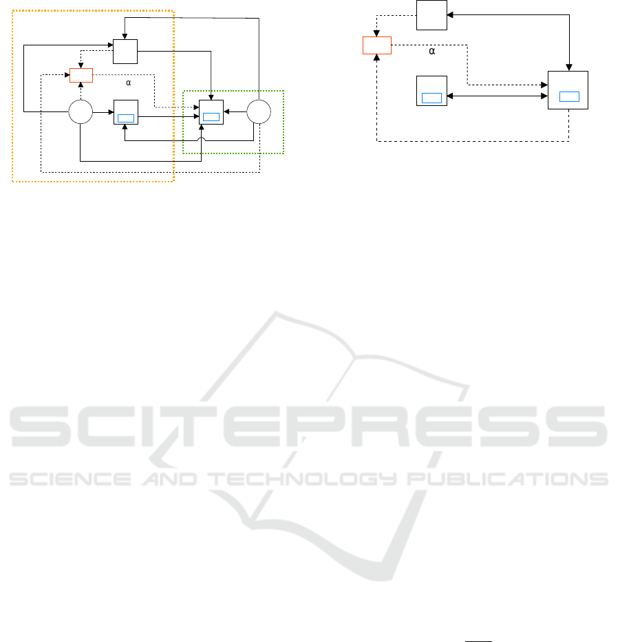
2.1.1 The Basic MG Architecture

The basic MG architecture, as shown in Fig. 1, rep-

resents the docked e-boat with the engine off, in the

generic timeslot k. On the left side, all the dock ele-

ments are enclosed in an orange rectangle, while the

elements related to the e-boat are enclosed in a green

rectangle.

Node N represents the Main Grid, G is the PV gener-

ator, S is the dock ESS, S

is the e-boat ESS and G

the e-boat PV roof. The elements named as BMS and

EMS stand for “Battery Management System” and

FCTA 2022 - 14th International Conference on Fuzzy Computation Theory and Applications

200

EMS

BMS

NS'

GS'

SS'

Dock

E-boat

G'S'

G'*

G'N

GS'

BMS

Figure 1: The basic MG architecture.

“Energy Management System”, respectively. Square

nodes are bidirectional, since energy can both ﬂow

from and to them. Circle nodes can only provide or

receive energy from other nodes. Regardless a node

is bidirectional or not, it can not both absorb/store

energy from or generate/provide energy to the other

nodes, in the same timeslot k. The BMS, which mea-

sures the State of Energy (SoE) of the ESS, is simu-

lated in a workstation, running also the FIS optimiza-

tion procedure. Energy ﬂows are drawn as solid black

lines in Fig. 1. The amount of energy which ﬂows

from the generic node i to the generic node j is indi-

cated as E

i j

. Thus, for example, E

is the amount

of energy which ﬂows from N to S

, during timeslot.

The nodes G and G

primarily meet the energy needs

of S

. In fact, conveying energy from S, assuming that

the dock ESS had been charged by G or G

, would

involve an additional operational cost due to the dock

ESS wear. Furthermore, it would be useless to route

the energy produced by G or G

to the Main Grid,

since that energy is primarily necessary to the e-boat

ESS. As a consequence, S and N should not receive

energy from S

but only from G and G

. The MG in-

formation ﬂows, drawn as dotted black lines in Fig. 1,

are the following: the whole energy produced by G in

the generic timeslot E

∗

, the whole energy produced

by G

in the generic timeslot E

∗

, the Main Grid en-

ergy purchase price p

and the EMS decision variable

α, which controls whether S

receives the difference

between its energy demand and the whole PV pro-

duction (G and G

) from N or from S. It is assumed

that suitable smart meters collect the above mentioned

information.

2.1.2 Simpliﬁed MG Architecture

According to the aforementioned considerations, S

G and G

can be grouped in a single node S

G, as

in 2. Thus, the overall PV energy production in the

EMS

BMS

G+G'

S'G'G

BMS

Figure 2: The simpliﬁed MG architecture.

generic timeslot E

G+G

and p

are the two inputs of

the EMS and the decision variable α is the system

output.

2.2 System Objectives

The EMS is in charge of optimizing the MG energy

ﬂows for achieving both the minimum overall charg-

ing cost and the minimum charging time of the e-

boat ESS. The quicker the charging process is, the

more stressed the ESS will be and, as a consequence,

the more expensive the charging process will be be-

cause of the ESS wear cost. Moreover, the quicker

the charging process is, the higher the probability of

buying energy from the Main Grid in k is, since S, G

and G

could not provide enough energy to meet the

e-boat demand. For the above reasons, the presented

objectives are in contrast to each other, hence the one

at hand is a Multi-Objective Pareto Front problem to

face.

2.3 MG Sizing

According to the LIFE Project, the area dedicated to

the PV panels is about 15 [mq]. Thanks to the Euro-

pean Commission PVGIS tool (EC, 2020), an estima-

tion of the PV generator peak power can be done by

the (1):

P = 1

kW p

Aη (1)

where P is the PV generator peak power, in [kWp];

A is the area dedicated to the PV panels, in [mq] and

η is the PV panels efﬁciency. The (1) is generally

used to assess the PV panels peak power when it has

been not provided by the manufacturer yet. Thus, the

peak power is calculated assuming that the PV pan-

els generate a fraction (given by the efﬁciency) of the

power it would generate under the Standard Condi-

tions (i.e. 1000 W/m2 solar irradiance, a module tem-

perature of 25° C and a solar spectrum corresponding

to an air mass of 1.5). As speciﬁed in (Departement of

Energy, 2016), the crystalline Silicon PV panels efﬁ-

Synthesis of an Evolutionary Fuzzy Multi-objective Energy Management System for an Electric Boat

201

ciency is about 0.25 for single-crystal cells while is

roughly 0.20 for multi-crystalline cells. With the aim

of exploiting solar irradiation well throughout the day,

multi-crystalline cells are to be preferred so that η is

set to 0.20. Therefore, the PV generator peak power

is 3 [kWp]. By a similar reasoning, the e-boat PV roof

peak power is about 1, 5 [kWp], since the area of the

PV panels is 8 [mq]. The dock ESS capacity is set

to be equal to the e-boat ESS capacity, which is de-

signed to be 50 [kWh]. This choice guarantees that

the e-boat ESS could be always fully charged when

docked, being the initial dock ESS SoE the 80% of its

capacity while the initial e-boat ESS SoE the 20% of

the same quantity. The ESS (both for dock and e-boat)

charging/discharging energy bound is set to 5 [kWh],

according to the Tesla Powerwall technical features

(Tesla, 2019).

3 DATASET

The dataset consist in hourly PV generation and Main

Grid energy purchase prices ﬁgures for 2020. More

detailed information about data and sources are re-

ported below.

3.1 PV Generation

Through the PVGIS tool (EC, 2020), it is possible to

achieve an estimation of the hourly PV production

data for a given geographic position, which for the

LIFE Project is 44.442

◦

N,11.215

◦

W (Orbetello, Tu-

cany, IT). PVGIS tool input values for the dock PV

generator include the peak power of about 3 kWp,

system loss (e.g. from cables) of about 14% and

slope/azimuth ﬁgures.

In particular, system loss (for example, losses in ca-

bles, power inverters and dirt on the PV modules) to-

gether with the Slope (angle of the PV modules from

the horizontal plane) are set by default, while the Az-

imuth (the angle of the PV modules relative to South)

is set for a perfect orientation to South. PVGIS tool

input values for the dock PV generator include the

peak power of about 1.5 kWp, system loss (e.g. from

cables) of about 14% and slope/azimuth ﬁgures,

whereslope is set to 0 degrees because the e-boat PV

roof is in a ﬁxed position, parallel to the deck.

3.2 Energy Purchase Prices

The Main Grid energy purchase prices come from

the Open Power System Data (Z

urich, 2020). More

precisely, data pertain the Center of Italy (where the

LIFE Project area is located), for 2020.

3.3 Dataset Analysis

Figures about energy purchase prices for 2020 are

available only until 1

October 2020, therefore, the

dataset consists of nine months of data, until the end

of September 2020. Since the e-boat is designed to

operate mainly during peak season, the dataset times-

pan is acceptable. No other lack of data is observed.

4 PROBLEM FORMULATION

The problem formulation consists of the following

equations:

min

k,α ε R

∑

k=1

(1 − SoE

)

(2)

min

k,α ε R

∑

k=1

+ w

+ c

buy

)

(3)

where:

T ≥ k ≥ 0 (4)

1 ≥ α ≥ 0 (5)

1 ≥ SoE

≥ 0 (6)

1 ≥ SoE

≥ 0 (7)



SoE

− 0.5

0.5



(8)



SoE

− 0.5

0.5



(9)

buy

(

0 i f E

≤ 0

i f E

> 0

(10)

+ E

= 0 (11)











max

0.49

− E

max

i f α ≤ 0.49

(α − 0.50)

max

0.50

i f α ≥ 0.50

(12)











−E

i f α ≤ 0.49

and |E

| < E

Smax

− |E

| i f α ≥ 0.50

and |E

| ≥ E

Smax

0 i f α ≥ 0.50

and |E

| < E

Smax

(13)

FCTA 2022 - 14th International Conference on Fuzzy Computation Theory and Applications

202











0 i f α ≤ 0.49

−E

i f α ≥ 0.50

and |E

| < E

Smax

−E

Smax

i f α1 ≥ 0.50

and |E

| ≥ E

Smax

(14)

max

= E

Smax

= 5 (15)

= C = 50 (16)

SoE

= SoE

k−1

−

(17)

SoE

= SoE

k−1

−

(18)

The EMS minimizes two Objective Functions (OFs).

The ﬁst OF, given in (2), is the sum of the e-boat

ESS capacity fractions that are full of energy, over

the whole dataset (T is the total number of times-

lots k and SoE

is the e-boat ESS State of Energy,

bounded as in (6). Minimizing the OF (2) means

maximizing the number of timeslots the e-boat ESS

is full, i.e. minimizing the ESS charging time. The

second OF is the sum of the overall MG costs over

the whole dataset, i.e. the e-boat ESS wear cost w

given by (8), the dock ESS wear cost w

given by

(9) and the Main Grid energy purchase c

buy

given by

(10). The ESS wear cost formulation comes from

(Ferrandino et al., 2020) such that the more the SoE

deviates from the 50% of the capacity the more the

battery is stressed. The energy purchase cost is con-

sidered everytime there is an energy ﬂow from the

Main Grid, that fore every k where E

is positive.

In fact, conventionally, a positive amount of energy

for a given node of the MG means that it is provid-

ing energy, while a negative amount means that it is

receiving energy. Thus, when E

is positive, c

buy

the product of E

for the energy purchase price at k.

The MG energy balance is guaranteed by (11). The

EMS output (or decision variable) α is a real-valued

number that is rounded to the second decimal place.

It is in charge of deciding both the amount of energy

to store in the e-boat ESS in k, as shown in (12), and

the node the e-boat ESS can mainly receive energy

from, by ( 13) and (14). More precisely, if α is less

than or equal to 0.49, the e-boat ESS stores energy

never over its technical limit (E

max

) by (12) and it

charges itself primarily from G and G

before relying

on N by (13) (i.e. E

is negative). With the afore-

mentioned condition on α in k, S does not exchange

any energy. On the other hand, if α is greater than or

equal to 0.50, the e-boat ESS stores energy never over

its technical limit (E

Smax

) by (12) and it charges itself

primarily from G and G

before relying on S by (14)

(i.e. E

is negative). That said, if the amount of

energy E

exceeds E

Smax

, the difference between

the former and the latter is provided by N, by (13).

With similar reasoning, again by (13) and (14), S and

N receive energy from S

G, if the energy balance of

the former is positive. The values of E

max

and E

Smax

are set by (15), according to Section 2.3, as it is for

the ESSs capacity, by (16). Furthermore, timeslot by

timeslot, the SoE of the ESSs is updated by (17) and

(18).

5 THE FIS-GA OPTIMIZATION

In a FIS-GA optimization (De Santis et al., 2013), (De

Santis et al., 2017), the FIS parameters are properly

set by a GA to achieve the problem objectives. In

the following, more details are given about the opti-

mization procedure performed in this work. Accord-

ing to the FIS-HGA paradigm (De Santis et al., 2017),

the GA can control which Rules to delete in the Rule

Base. This feature is useful fore achieving the core of

the most relevant Rules for the problem at hand. Each

one of these new Genes represents the presence or ab-

sence of a MF such that, if the MF is absent, the Rules

with that MF are deleted. The aforementioned Genes

are called Hierarchical Genes. The generic HGA In-

dividual can be represented as follows:

= [~g

, ~g

] (19)

where ~g

is the vector of the binary Hierarchical

Genes, ~g

is the vector of Antecedents,

F encodes

the MF abscissas, ~g

is the vector of Consequents and

encodes Rule Weights.

5.1 Design of the MO-FIS-HGA

Algorithm

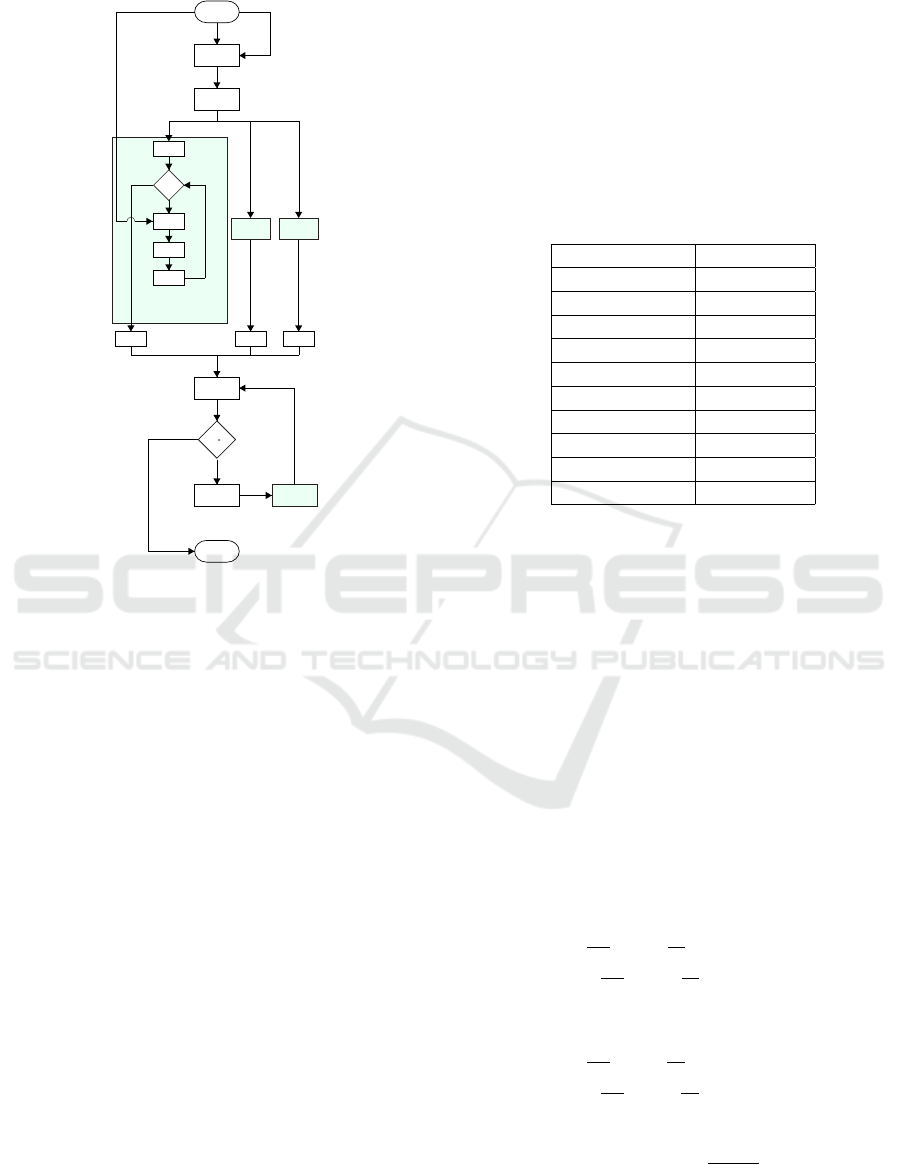
5.1.1 Optimization Workﬂow

A MO-FIS-HGA optimization algorithm returns the

optimal FIS models that belong to the Pareto Front.

In fact, as speciﬁed in Subsection 2.2, two OFs, in

contrast to each other, are considered. The optimiza-

tion workﬂow is presented in Fig. 3.

5.1.2 FIS Design

A Mamdami-type FIS consists of 25 Rules in the Rule

Base and a ﬁve MFs Term set, for both the two Inputs

Synthesis of an Evolutionary Fuzzy Multi-objective Energy Management System for an Electric Boat

203

START

GA encoding

initialization

GA decoding

OF evaluation

process

OF evaluation

process

...

OF evaluation

process

...

GA Selection

END

GA Crossover

& Mutation

OF evaluation

process

far all Individuals

k Simulation timeslot

Population bounds

Base FIS structure

Initial Population

Individual 1

FIS structure

Individual N

FIS structure

k = 1

sum = 0

k <= T?

True

k++

Output ( )

False

FIS evaluation

Energy

balance

sum = sum +

OF = sumOF = sum OF = sumOF = sum OF = sum

New Population

Initial Population-FO

matrix

Old Population

Individual ...

FIS structure

Population size

ΔT

Time horizon (dataset length)

k+1

Input (E

GG'

; p

k+1

)

k+1

check and

SoE update

Max number of

genera

ons

reached ?

True

False

GA Elitism

Pareto Front

(Optimized FIS

structures)

Figure 3: Optimization ﬂowchart.

and the Output. The number of Rules comes from

(20):

= n

MFs

(20)

where n

is the number of Rules, n

is the number of

Inputs (2, in this case) and n

MFs

is the number of MFs

in the Term Set (5 in this case).

5.1.3 HGA Design

The MO-HGA encodes Consequents and Weights as

Genes of its Individuals and the generic current Popu-

lation evolves, generation by generation, with the aim

of ﬁnding a PF trade-off between the two OFs. In-

spired by (Dietz et al., 2008), at ﬁrst, the GA ﬁnds

the Individuals with the minimum values of the two

OFs. This Elitism procedure aims at covering the PF

edges. Then, two Selection processes are performed:

the ﬁrst one, considering the ﬁrst OF and the second

one considering the second OF. That leads to achieve

two groups of Individuals: the ﬁrst one, containing

Individuals from the ﬁrst Selection (i.e. with good

values for the ﬁrst OF); the second one, as large as

the ﬁrst one, containing Individuals from the second

Selection (i.e. with good values for the second OF), ﬁ-

nally performing a crossover between the Individuals

of the aforementioned groups. This practice ‘breeds’

Individuals in a way that, Generation by Generation,

the probability that they will reach the inner part of the

Pareto Front increases. Then, Mutation is applied to

remaining Individuals of the current Population, lead-

ing to the updated Population completion and, thus,

to a new Generation. The HGA operators and meta-

parameters, which are set by the operator based on

previous experience on this kind of applications, are

shown in Tab. 1.

Table 1: HGA operators and meta-parameters.

Figure Value

Pop. size 300

Elite Indiv. 1 (per OF)

Selection Op. Tournament

Sel. Tour. size 2

Mutation Op. Uniform

Mut. Fraction 0.2

Crossover Op. One-point

Cros. Fraction 0.8

Stopping cond. Max. Gen.

Max Gen. 50

FIS MFs abscissas are encoded as Genes but further

transformations are done with the aim of reducing the

number of Genes and, therefore, the computational

cost. First of all, the UoD is discretized with 0.01

steps. Then, MFs abscissas are encoded following the

(21 - 35) . With reference to Fig. 4, even if each

triangular MF counts three abscissas, only two real

values are needed, according to the aforementioned

equations and inequalities.

γ = g

very low

(21)

β = g

very low

γ (22)

θ = g

very high

(1 − θ

) (23)

λ = θ + g

very high

(1 − θ) (24)

φ =







− (

l ow

low

−

) i f g

low

≥ 1

+ (−

l ow

low

) i f 0.01 ≥ g

low

< 1

(25)

ξ =







+ (

l ow

low

−

) i f g

low

≥ 1

− (−

l ow

low

) i f 0.01 ≥ g

low

< 1

(26)

ω = φ + g

low

(ξ − φ)

(27)

FCTA 2022 - 14th International Conference on Fuzzy Computation Theory and Applications

204

with

= 0.25 (28)

= 0.75 (29)

0.04 ≥ g

very low

≤ 4.00 (30)

0.01 ≥ g

very low

≤ 0.99 (31)

0.04 ≥ g

very high

≤ 4.00 (32)

0.01 ≥ g

very high

≤ 0.99 (33)

0.01 ≥ g

low

≤

(34)

0.01 ≥ g

low

≤ 1.99 (35)

where γ, β, θ, λ, φ, ξ and ω are the MFs abscissas

(Fig. 4), being γ

, β

, θ

, λ

, φ

, ξ

and ω

their de-

fault values; g

very low

and g

very low

are the ﬁrst and the

second Genes for the “very low” trapezoidal MF, re-

spectively; g

very high

and g

very high

are the ﬁrst and the

second Genes for the “very high” trapezoidal MF, re-

spectively; g

low

and g

low

are the ﬁrst and the second

Genes for the “low” triangular MF, respectively. The

“low” triangular MF is to be considered representa-

tive of the others triangular MFs; thus, for the sake of

the synthesis, the values of φ

, ξ

and ω

are omitted

in the equations above. The equations and inequal-

ities above guarantee MFs abscissas variations over

the whole UoV also preventing overlaps. This way,

the number of MFs abscissas Genes is 30 (3 overall

Terms Sets - for 2 Inputs and 1 Output - for 5 MFs

per Term Set for 2 Genes per MF) instead of 39 (3

overall Terms Sets - for 2 Inputs and 1 Output - for

5 MFs per Term Set for 2 Genes per trapezoidal MF

and 3 Genes per triangular MF.).

As discussed above, the generic Individual counts 90

Genes: 10 Hierarchical Genes (1 per Input MF for 5

MFs per per Input Term Set for 2 Input Term Sert); 30

MFs Genes; 25 Consequents Genes (1 per Rule for 25

Rules); 25 Weight Genes(1 per Rule for 25 Rules).

5.2 Benchmark and Performance

Metrics

A Dynamic Programming (DP) algorithm is used

as benchmark in this work. According to Litera-

ture (Kim and de Weck, 2005), (Koski, 1985), a

benchmark PF can be achieved by implementing a

mono-objective algorithm with a single weighted-

sum OF, by ﬁnding problem solutions for many differ-

ent weights values. In this work, 100 different bench-

mark PF points are achieved by the above procedure.

Figure 4: MF encoding scheme.

With regard to the performance metrics, the following

criteria must be taken into account for a MO optimiza-

tion (Chen et al., 2007), (Unveren and Acan, 2007):

• Proximity of the GA PF points the to the bench-

mark PF points;

• Coverage of the benchmark PF by the GA PF

points;

• Distribution of the GA PF points.

Proximity can be estimated through the Genera-

tional Distance (GD) (Unveren and Acan, 2007), as

follows:

GD =

∑

(36)

where z

is the distance between the i-th GA PF point

and its nearest benchmark PF point and M is the total

number of GA PF points. If GD is 0, GA PF points

overlap with the benchmark PF points.

Both coverage and distribution can be evaluated

through the Diversity Metric (DM) (Chen et al.,

2007), (Unveren and Acan, 2007), with reference to

Fig. 5, as follows:

DM =

+ d

∑

M−1

−

+ d

+ (M − 1)

(37)

where d

and b

are the distance between the extreme

GA PF points and the corresponding points in the

benchmark PF, while d

and

d are the distance be-

tween two consecutive GA PF points and their mean

value, respectively. It can be seen that the more the

mutual distance between GA PF points is closer to

and the distances d

and d

are small, the more DM

tends to 0, which means a perfect GA PF points cov-

ering and distribution.

Synthesis of an Evolutionary Fuzzy Multi-objective Energy Management System for an Electric Boat

205

According to (Chen et al., 2007) and (Unveren and

Acan, 2007), values of GD up to about 0.45 and val-

ues of DM up to about 0.40 are acceptable.

OF1

OF2

GA PF point

DP PF point

Figure 5: Density Metric (DM) calculation quantities.

6 TESTS AND RESULTS

In order to achieve the optimal FIS models with the

best generalization skills, a k-fold cross-validation is

performed by choosing 5 couples of days (5-fold) in

the dataset trying to cover as much as possible the

whole year. Therefore, each couple consists of one

training day subset and one validation day subset and

the PF solutions (i.e. the optimal FIS models) with

the minimum validation error are selected before be-

ing tested on one day, randomly chosen in the dataset.

More precisely, the error ε is calculated as the sum

of GD and DM performance metrics (38), aiming at

guaranteeing both accuracy and a good PF points dis-

tribution. In fact, the aforementioned sum of perfor-

mance metrics acts as weighted-sum objective func-

tion with equal given both to GD and DM, aspiring at

a good compromise result.

ε = GD + DM (38)

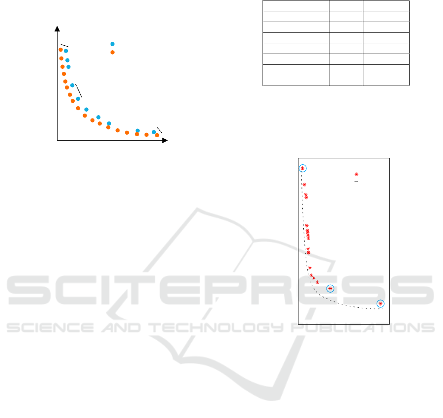
The result of the learning process is the optimal GA

PF, which consists of the best FIS models for the

problem at hand. The optimal GA PF is plotted

against the benchmark PF in Fig. 6 and ﬁgures about

the algorithm performance are reported in Tab. 2.

Since the GA is a stochastic algorithm, the values in

Tab. 2 are calculated as averages over 10 runs.

At the best of our knowledge, the proposed algorithm

achieves acceptable results in GD ﬁgures but also

promising values of DM, if compared to other GA-

based algorithms (Unveren and Acan, 2007), (Chen

et al., 2007). That could be encouraging for further

improvements of the model.

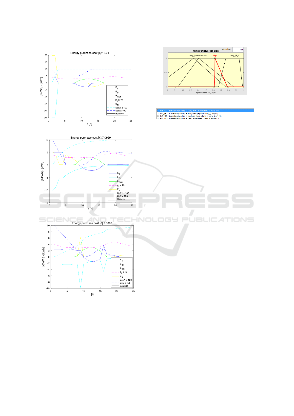
For three GA PF points, (i.e. FIS models), the result-

ing optimal energy ﬂows are extracted and shown in

Fig. 7, together with an estimation of the energy pur-

chase cost from the Main Grid. The points are chosen

Table 2: MO-FIS-HGA performance metrics.

Figure Mean Variance

Train. GD 0.062 0.002

Train. DM 0.162 0.0013

Val. GD 0.076 0.009

Val. DM 0.162 0.004

Test. GD 0.063 0.009

Test. DM 0.164 0.009

Comp. cost [h] 6.320 0.005

to be the two extreme points of the PF and the one in

the middle (Fig. 6) because in a MO optimization it

is interesting to study both the sharp and the compro-

mise solutions, in order to choose the most suitable

one.

III

0.05 0.1 0.15 0.2 0.25 0.3 0.35 0.4 0.45

0.4

0.6

0.8

1.2

1.4

1.6

OF1

FIS-HGA

Figure 6: FIS-HGA Pareto Front selected points.

In the Point I case, for a faster e-boat ESS charge

(about 2 hours), the dock ESS immediately transfers

as much energy as possible to the e-boat ESS, accord-

ing to its technical limits. The larger energy contribu-

tion comes from the Main Grid, with an energy pur-

chase cost that is the higher among the overall cases.

In the opposite case of Point III, a very smaller quan-

tity of energy is absorbed by the e-boat from the Main

Grid, with about a purchase costs less than about the

85%. Moreover, solar energy is exploited to charge

both the e-boat ESS and the dock ESS. That makes it

possible to buy less energy from the Main Grid than

in the other cases and also to charge less rapidly, with

a lower stress for the ESSs (it is better if an ESS SoE

is around 50%). As a consequence, the e-boat ESS is

not fully charged (about 90%) and it takes the whole

day to ﬁnish charging. In a compromise solution, in

the Point II case, the energy purchase costs are less

than the 50% if compared to Point I case and at 12

o’clock it is almost fully charged (about 80%). The

last case can be considered the best in terms of lo-

FCTA 2022 - 14th International Conference on Fuzzy Computation Theory and Applications

206

Point I

Point II

Point III

Figure 7: Optimal energy ﬂows from delected FIS-HGA

Pareto Front points.

gistic and economic points of view, so the ﬁrst Input

Term Set (as an example) of the corresponding FIS

model (Fig. 8) are discussed below for the sake of the

AI Explainability.

Together with the Rule Set (Fig. 9) the Term Sets

make the FIS reasoning comprehensible to humans,

in contrast with AI black-box models.

Figure 8: Point II FIS Term Set for the ﬁrst Input.

Figure 9: Point II FIS Rule Base excerpt.

7 CONCLUSIONS

An MO EMS is synthesized for a docked e-boat with

the aim of optimizing two conﬂicting objective func-

tions, i.e. charging the e-boat ESS as soon as possi-

ble within 24h and spending as little as possible both

for energy purchase from the Main Grid and also in

terms of ESS wear. A FIS-HGA algorithm is used to

achieve the Pareto Front for evaluating compromise

solutions. The HGA is in charge of optimizing the

FIS parameters in order to return a FIS model that

meets the needs. Five k-fold, each with one train-

ing and one validation day dataset, are considered for

cross-validation. Results laid to a balanced trade-off

between the two objectives, since the selected solu-

tion make it possible to charge the e-boat ESS in a

reasonable time for people transportation services (it

is almost fully charged at 12 o’ clock) with an over-

all expenditure that is less than 50%, if compared to

the most expensive solution. Having a FIS model as

a function approximation model makes it possible to

know its reasoning process by observing Term Set

and Rule Base, since they are written in a Natural-like

Language. The proposed algorithm achieves good re-

sults in DM ﬁgures while only acceptable ﬁgures in

GD, if compared to literature. That could be encour-

aging for further improvements of the model. One of

the model ﬂaws is the high computational cost that

requires efforts in writing more efﬁcient code and in

exploiting better parallel computation.

REFERENCES

Alsharif, A., Tan, C. W., Ayop, R., A.Dobi, and Lau, K. Y.

(2021). A comprehensive review of energy manage-

ment strategy in vehicle-to-grid technology integrated

with renewable energy sources. Sustainable Energy

Technologies and Assessments, 47:101439.

Synthesis of an Evolutionary Fuzzy Multi-objective Energy Management System for an Electric Boat

207

Badal, F., Das, P., and et al., S. S. (2019). A survey on

control issues in renewable energy integration and mi-

crogrid. Protection and Control of Modern Power Sys-

tems, 4.

Balestra, L. and Schjølberg, I. (2021). Energy manage-

ment strategies for a zero-emission hybrid domes-

tic ferry. International Journal of Hydrogen Energy,

46(77):38490–38503.

Capillo, A., Luzi, M., Pasc, M., Rizzi, A., and Mascioli, F.

M. F. (2018). Energy transduction optimization of a

wave energy converter by evolutionary algorithms. In

2018 International Joint Conference on Neural Net-

works (IJCNN), pages 1–8.

Chen, L., McPhee, J., and Yeh, W. W.-G. (2007). A diver-

siﬁed multiobjective ga for optimizing reservoir rule

curves. Advances in Water Resources, 30(5):1082–

1093.

De Santis, E., Rizzi, A., and Sadeghian, A. (2017). Hier-

archical genetic optimization of a fuzzy logic system

for energy ﬂows management in microgrids. Applied

Soft Computing, 60:135–149.

De Santis, E., Rizzi, A., Sadeghiany, A., and Frattale

Mascioli, F. M. (2013). Genetic optimization of a

fuzzy control system for energy ﬂow management in

micro-grids. In 2013 Joint IFSA World Congress and

NAFIPS Annual Meeting (IFSA/NAFIPS), pages 418–

423.

Departement of Energy, U. (2016). Crystalline silicon pho-

tovoltaic research. http://www.energy.gov/eere/solar/

crystalline-silicon-photovoltaics-research.

Dietz, A., Azzaro-Pantel, C., Pibouleau, L., and Domenech,

S. (2008). Strategies for multiobjective genetic al-

gorithm development: Application to optimal batch

plant design in process systems engineering. Comput-

ers & Industrial Engineering, 54(3):539–569.

Duman, A. C., Erden, H. S.,

Omer G

ul, and

Onder

uler (2021). A home energy management system

with an integrated smart thermostat for demand re-

sponse in smart grids. Sustainable Cities and Society,

65:102639.

EC (2020). Photovoltaic geographical information system.

http://re.jrc.ec.europa.eu/pvg tools/en/.

Ellabban, O., H.Abu-Rub, and Blaabjerg, F. (2014). Renew-

able energy resources: Current status, future prospects

and their enabling technology. Renewable and Sus-

tainable Energy Reviews, 39:748–764.

Ferrandino, E., Capillo, A., Frattale Mascioli, F. M., and

Rizzi, A. (2020). Nanogrids: A smart way to inte-

grate public transportation electric vehicles into smart

grids. In 12th International Joint Conference on Com-

putational Intelligence, volume 16.

Haﬁz Abdul Muqeet, a. H. M. M., Javed, H., Shahzad, M.,

Jamil, M., and Guerrero, J. M. (2021). An energy

management system of campus microgrids: State-of-

the-art and future challenges. Energies, 14(20).

Kim, I. and de Weck, O. (2005). Adaptive weighted-sum

method for bi-objective optimization: Pareto front

generation. Structural and Multidisciplinary Opti-

mization, 29(2):149–158.

Koski, J. (1985). Defectiveness of weighting method in

multicriterion optimization of structures. Communi-

cations in Applied Numerical Methods, 1(6):333–337.

Layton, B. E. (2008). A comparison of energy densities of

prevalent energy sources in units of joules per cubic

meter. International Journal of Green Energy, 5:438–

455.

Li, X.-H., Cao, C. C., Shi, Y., Bai, W., Gao, H., Qiu, L.,

Wang, C., Gao, Y., Zhang, S., Xue, X., and Chen, L.

(2022). A survey of data-driven and knowledge-aware

explainable ai. IEEE Transactions on Knowledge and

Data Engineering, 34(1):29–49.

Palm, R. (2004). Synchronization of decentralized multiple-

model systems by market-based optimization. IEEE

Transactions on Systems, Man, and Cybernetics, Part

B (Cybernetics), 34(1):665–671.

Pozna, C., Precup, R.-E., Horvath, E., and Petriu, E. M.

(2022). Hybrid particle ﬁlter-particle swarm opti-

mization algorithm and application to fuzzy controlled

servo systems. IEEE Transactions on Fuzzy Systems,

pages 1–1.

Raﬁei, M., Boudjadar, J., and Khooban, M.-H. (2021). En-

ergy management of a zero-emission ferry boat with a

fuel-cell-based hybrid energy system: Feasibility as-

sessment. IEEE Transactions on Industrial Electron-

ics, 68(2):1739–1748.

Slama, S. B. (2021). Design and implementation of home

energy management system using vehicle to home

(h2v) approach. Journal of Cleaner Production,

312:127792.

Tesla (2019). Pawerwall 2 datasheet. http://www.tesla.com/

powerwall.

Unveren, A. and Acan, A. (2007). Multi-objective optimiza-

tion with cross entropy method: Stochastic learning

with clustered pareto fronts. In 2007 IEEE Congress

on Evolutionary Computation, pages 3065–3071.

Xiang, Y. and Yang, X. (2021). An ecms for multi-objective

energy management strategy of parallel diesel electric

hybrid ship based on ant colony optimization algo-

rithm. Energies, 14(4).

Zamﬁrache, I. A., Precup, R.-E., Roman, R.-C., and Petriu,

E. M. (2022). Reinforcement learning-based control

using q-learning and gravitational search algorithm

with experimental validation on a nonlinear servo sys-

tem. Information Sciences, 583:99–120.

Ozdemir, H., G

uldorum, H. C., Erdinc¸, O., and

Ibrahim

S¸eng

or (2021). Energy management of a port serv-

ing fuel cell and battery based hybrid green ferries. In

2021 International Conference on Smart Energy Sys-

tems and Technologies (SEST), pages 1–6.

urich, E. (2020). Open power system data. http://data.

open-power-system-data.org/time series/.

FCTA 2022 - 14th International Conference on Fuzzy Computation Theory and Applications

208