
Degree Centrality Algorithms for Homogeneous Multilayer Networks
Hamza Reza Pavel, Abhishek Santra and Sharma Chakravarthy
Computer Science and Engineering Department and, Information Technology Laboratory (IT Lab),
The University of Texas at Arlington, Arlington, Texas 76019, U.S.A.
Keywords:
Homogeneous Multilayer Networks, Degree Centrality, Decoupling Approach, Accuracy & Precision.
Abstract:
Centrality measures for simple graphs/networks are well-defined and each has numerous main-memory al-
gorithms. However, for modeling complex data sets with multiple types of entities and relationships, simple
graphs are not ideal. MultiLayer Networks (or MLNs) have been proposed for modeling them and have been
shown to be better suited in many ways. Since there are no algorithms for computing centrality measures
directly on MLNs, existing strategies reduce (aggregate or collapse) MLN layers to simple networks using
Boolean AND or OR operators. This approach negates the benefits of MLN modeling as these computations
tend to be expensive and furthermore results in loss of structure and semantics.
In this paper, we propose heuristic-based algorithms for computing centrality measures (specifically, de-
gree centrality) on MLNs directly (i.e., without reducing them to simple graphs) using a newly-proposed
decoupling-based approach which is efficient as well as structure and semantics preserving. We propose mul-
tiple heuristics to calculate the degree centrality using the network decoupling-based approach and compare
accuracy and precision with Boolean OR aggregated Homogeneous MLNs (HoMLNs) for ground truth. The
network decoupling approach can take advantage of parallelism and is more efficient compared to aggregation-
based approaches. Extensive experimental analysis is performed on large synthetic and real-world data sets of
varying graph characteristics to validate the accuracy, precision, and efficiency of our proposed algorithms.
1 INTRODUCTION
In graph-based applications, an important require-
ment is to measure the importance of a node/vertex,
which can translate to meaningful real-world infer-
ences on the data set. For example, cities that act
as airline hubs, people on social networks who can
maximize the reach of an advertisement/tweet/post,
identification of mobile towers whose malfunction-
ing can lead to the maximum disruption, and so on.
Centrality measures include degree centrality (Br
´
odka
et al., 2011), closeness centrality (Cohen et al., 2014),
eigenvector centrality (Sol
´
a et al., 2013), stress cen-
trality (Shi and Zhang, 2011), betweenness centrality
(Brandes, 2001), harmonic centrality (Boldi and Vi-
gna, 2014), and PageRank centrality (Pedroche et al.,
2016), are some of the well-defined and widely-used
local and global centrality measures.
These centrality measurements use a set of crite-
ria to determine the importance of a node or edge in
a graph. Degree centrality metric measures the im-
portance of a node in a graph in terms of its degree,
which is the number of 1-hop neighbors a node has in
the graph. Most centrality metrics are clearly defined
for simple graphs or monographs or networks, and
there are numerous techniques for calculating them
on simple graphs. However, for modeling complex
data sets with multiple types of entities and relation-
ships, multilayer networks have been shown to be a
better alternative due to the clarity of representation,
ability to preserve the structure and semantics of dif-
ferent types of relationships for the same and different
sets of nodes, and support efficient computation using
parallelism (Kivel
¨
a et al., 2014; Santra et al., 2017b;
Fortunato and Castellano, 2009).
A multilayer network (De Domenico et al., 2013;
Santra and Bhowmick, 2017; Santra et al., 2020)
is made up of layers, each of which is a simple
graph or a network with nodes (that correspond to
entities) and edges (that correspond to relationships).
Nodes within a layer are connected (termed intra-
layer edges) based on a relationship between nodes.
Nodes in a layer may also be optionally connected to
nodes in other layers through inter-layer edges. As
an example, the diverse interactions among the same
set of people across different social media (such as
Facebook, LinkedIn, and Twitter) can be modeled
using a multilayer network (see Figure 1.) In this
Pavel, H., Santra, A. and Chakravarthy, S.
Degree Centrality Algorithms for Homogeneous Multilayer Networks.
DOI: 10.5220/0011528900003335
In Proceedings of the 14th International Joint Conference on Knowledge Discovery, Knowledge Engineering and Knowledge Management (IC3K 2022) - Volume 1: KDIR, pages 51-62
ISBN: 978-989-758-614-9; ISSN: 2184-3228
Copyright
c
2022 by SCITEPRESS – Science and Technology Publications, Lda. All rights reserved
51

MLN, the entities in each layer are the same, but the
relationships in each layer are different (Facebook-
friends, Twitter-relationships, LinkedIn-connections),
this sort of MLN is referred to as homogeneous MLNs
(or HoMLNs). As and the edges between layers are
implicit, they are not shown. It is also feasible to build
MLNs with different types of entities and relation-
ships within and between layers. This form of het-
erogeneous MLNs (or HeMLNs) is required for mod-
eling, for example, the DBLP data set (dbl, ) with au-
thors, articles, and conferences (Kivel
¨
a et al., 2014).
Hybrid Multilayer networks (HyMLNs) include both
types of layers.
Figure 1: Social Media HoMLN Example.
For a social-network HoMLN such as the one
shown in Figure 1, it will be interesting to find out
the set of people who are the most influential in a
single network or across multiple (or a subset of) so-
cial networks. This corresponds to finding out the de-
gree centrality nodes of a MLN using one or more
layers. Since extant algorithms that calculate degree
centrality measures on networks are limited to sim-
ple graphs/networks, MLNs need to be converted (us-
ing aggregation or projection) to simple graphs which
leads to the loss of structure and semantics. This pa-
per presents heuristic-based algorithms for computing
degree centrality nodes (or DC nodes) on HoMLNs
directly with high accuracy/precision and efficiency.
Boolean OR composition of layers is used for ground
truth in this paper.
For comparing the accuracy and precision of the
decoupling-based algorithms, we use Boolean opera-
tors for aggregation of layers and use simple graph al-
gorithms on them for ground truth. Other types of ag-
gregations are also possible. The aggregation of lay-
ers using AND and OR Boolean operators for homo-
geneous MLNs are straightforward as the nodes are
the same in each layer and the Boolean operator se-
mantics are applied to the edges. Both AND and OR
operators are commutative and distributive. OR ag-
gregation is likely to increase the size of the graph
(number of edges) used for ground truth. Accuracy is
computed by comparing the ground truth results for
the graph with the results obtained by the decoupling-
based algorithm for the layers of the same graph. The
naive algorithm uses only the results of each layer for
the computation (in this case degree centrality) and
applies the Boolean operator to the individual results
during the composition step. Typically, the naive ap-
proach does not yield good accuracy requiring addi-
tional information from each layer to be retained and
used for the composition algorithm using heuristics.
As layers are processed independently (may be in par-
allel), no information about the other layer is assumed
while processing a layer.
We adapt the decoupling-based approach pro-
posed in (Santra et al., 2017a; Santra et al., 2017b)
for our algorithms. Based on this approach, we com-
pute centrality on each layer independently once and
keep minimal additional information from each layer
for composing. With this, we can efficiently estimate
the degree centrality (DC) nodes of the HoMLN. This
approach has been shown to be application indepen-
dent, efficient, lends itself to parallel processing (of
each layer), and is flexible for computing centrality
measures on any subset of layers. The naive approach
to which we compare our proposed heuristic-based
accuracy and precision retains no additional informa-
tion from the layers apart from the degree centrality
nodes and their values. Contributions of this paper
are:
• Algorithms for directly computing degree cen-
trality nodes of Homogeneous MLNs (HoMLNs.)
• Several heuristics to improve accuracy, preci-
sion, and efficiency of computed results
• Decoupling-based approach to preserve struc-
ture and semantics of MLNs
• Experimental analysis on large number of syn-
thetic and real-world graphs with diverse charac-
teristics
• Accuracy, Precision, and Efficiency compar-
isons with ground truth and naive approach
The rest of the paper is organized as follows: Sec-
tion 2 discusses related work. Section 3 introduces
the decoupling approach used for MLN analysis and
discusses its advantages and challenges. Section 4
discusses ground truth and naive approach to degree
centrality. Sections 5 and 6 describe composition-
based degree centrality computation for HoMLNs us-
ing heuristics for accuracy and precision, respectively.
Section 7.1 describes the experimental setup and the
KDIR 2022 - 14th International Conference on Knowledge Discovery and Information Retrieval
52

data sets. Section 7.2 discusses result analysis fol-
lowed by conclusions in Section 8.
2 RELATED WORK
As complex and massive real-world data sets are be-
coming more popular and accessible, there is a press-
ing need to model them using the best approach
and analyze them efficiently in various ways. How-
ever, use of graphs for their modeling and especially
MLNs poses additional challenges in terms of com-
puting centrality measures on MLNs instead of sim-
ple graphs. Centrality measures including MLN cen-
trality shed light on various properties of the network.
Although there have been numerous studies on rec-
ognizing central entities in simple graphs, there have
been few studies on detecting central entities in mul-
tilayer networks. Existing research for finding central
entities in multilayer networks is use-case specific,
and there is no standard paradigm for addressing the
problem of detecting central entities in a multilayer
network.
Degree centrality is the most common and widely-
used centrality measure. Degree centrality is used to
identify essential proteins (Tang et al., 2013). It is
also used in identifying epidemics in animals (Can-
deloro et al., 2016) and the response of medication
in children with epilepsy (Wang et al., 2021). The
most common and prominent use of degree central-
ity is in the domain of social network analysis. Some
of the common use of degree centrality in social net-
work analysis is identifying the most influential node
(Srinivas and Velusamy, 2015), influential spreaders
of information (Liu et al., 2016), finding opinion lead-
ers in a social network (Risselada et al., 2016), etc.
Despite being one of the most common and widely
used centrality measures, very few algorithms or solu-
tions exist to directly calculate the degree centrality of
a MLN. In this study (Br
´
odka et al., 2011), the author
proposes a solution to find degree centrality in a 10-
layer MLN consisting of the Web 2.0 social network
data set. Similar to the previous work, in (Rachman
et al., 2013), authors identify the degree centrality of
nodes using the Kretschmer method. The authors in
this study (Yang et al., 2014) proposed a node promi-
nence profile-based method to effectively predict the
degree centrality in a network. In another study (Gaye
et al., 2016), authors propose a solution to find the
top-K influential person in a MLN social network us-
ing diffusion probability. More recently there has
been some work in developing algorithms for MLNs
using the decoupling-based approach (Santra et al.,
2017b).
The majority of degree centrality computation al-
gorithms are main memory based and are not suit-
able for large graphs. They are also use-case spe-
cific. In this paper, we adapt a decoupling-based tech-
nique proposed in (Santra et al., 2017b) for MLNs,
where each layer can be analyzed individually and
in parallel, and graph characteristics (such as de-
gree centrality nodes) for a HoMLN can be cal-
culated utilizing the information gathered for each
layer. Our algorithms follow the network decoupling
methodology, which has been demonstrated to be effi-
cient, flexible, and scalable. Achieving desired accu-
racy/precision/recall, however, is the challenge. Our
approach is not strictly main-memory based as each
layer (which is likely to be smaller than the aggre-
gated graph) outputs results into a file which are used
for the decomposition algorithm. Also, as each layer
is likely to be smaller than the OR aggregation of lay-
ers, larger size MLNs can be accommodated in our
approach.
3 NETWORK DECOUPLING
APPROACH
Existing multilayer network analysis approaches con-
vert or transform a MLN into a simple graph
1
. Ag-
gregating or projecting the network layers into a sim-
ple graph accomplishes this. Edge aggregation is used
to bring homogeneous MLNs together into a simple
graph. Although aggregating a MLN into a simple
network enables the use of currently available tech-
niques for centrality and community discovery (of
which there are many), the MLN structure and se-
mantics are not retained, causing information loss.
We use the network decoupling strategy for MLN
analysis to overcome the aforementioned difficulties.
Figure 2 shows the proposed network decoupling
strategy. It entails determining two functions: one
for analysis (Ψ) and the other for composition (Θ).
Each layer is analyzed independently using the anal-
ysis function (and in parallel). The partial results (as
they are called) from each of the two layers are then
combined using a composition function/algorithm to
obtain the HoMLN results for the two layers. MLNs
with more than two layers can use this binary com-
position repeatedly. Independent analysis permits the
use of existing techniques for each layer. Decoupling,
on the other hand, increases efficiency, flexibility, and
scalability along with extending the existing graph
1
A simple graph has nodes that are connected by edges
(optionally labeled and/or directed) with no loops or multi-
ple edges between same odes.
Degree Centrality Algorithms for Homogeneous Multilayer Networks
53

Figure 2: Overview of the network decoupling approach.
analysis algorithms to compute directly on MLNs.
As the network decoupling method preserves the
structure and semantics of the data, drill-down and vi-
sualization of final results are easy to support. Each
layer (or graph) is likely to be smaller, consume less
memory than the whole MLN, and composition is
done as a separate step on the partial results. The
analysis function results are preserved and used in
the composition. The requirement to recompute is re-
duced because the result of analysis for a layer can
be reused by several composition functions, increas-
ing the efficiency of the decoupling-based approach.
Individual layers can be analyzed using any of the
available simple graph centrality algorithms. This
method is also application-independent. As a result,
the decoupling-based approach can be used to extend
existing centrality algorithms to MLNs. To compose
the outputs of analysis functions (partial results) into
the final results, we only need to define the composi-
tion function.
The problem with a decoupling-based approach is
getting high accuracy when compared to the ground
truth. This translates to one of the major challenges
in determining the minimum additional information
to retain as part of the layer analysis step to be used
during composition to improve the overall accuracy
and precision with respect to the ground truth. For
many composition algorithms we have looked into,
there is a trade-off between using more information
from each layer and improving accuracy or precision.
This trade-off is demonstrated in this paper as well.
The decoupling approach’s layer-wise analysis
has a number of advantages. First, only a smaller
layer of the network needs to be loaded into memory,
rather than the whole network. Second, the analysis
of individual layers can be parallelized, reducing the
algorithm’s overall storage requirements and execu-
tion time. Finally, the composition function (Θ) relies
on intuition, which is built into the heuristic and takes
substantially less complex computationally than Ψ.
The accuracy of a MLN analysis algorithm is de-
termined by the information we keep (in addition to
the output) during individual layer analysis. The ba-
sic minimum information we may maintain from each
layer in terms of centrality measurements is the high
centrality nodes of that layer, as well as their central-
ity values. The accuracy should potentially improve
as we retain more relevant information for compo-
sition. However, determining what is relevant and
should be retained to improve accuracy or precision is
the main challenge of this approach. The key hurdles
are identifying the most beneficial minimal informa-
tion and the intuition for their effectiveness.
4 DEGREE CENTRALITY FOR
MLNs
The degree of a node in a graph is the total number
of edges that are incident on it
2
. Degree hubs are
nodes in a network that have a degree larger than
or equal to the network’s average degree. Degree
hubs are specified for simple graphs. In (Santra et al.,
2017b), the authors have proposed three algorithms
to estimate degree hubs in AND composed multilayer
networks. However, there are no algorithms for cal-
culating degree hubs for OR composed HoMLNs.
If the HoMLN layers are composed of a Boolean op-
eration such as OR, we can expand the notion of a hub
from a simple graph to HoMLNs. In this paper, we
suggest various composition functions to maximize
accuracy, precision, and efficiency while estimating
degree hubs in OR composed multilayer networks.
The ground truth is used to evaluate the perfor-
mance and accuracy of our suggested heuristics for
detecting the degree hubs of a multilayer network.
The degree centrality of a vertex u in a network
is defined as C
D
(u) = Number of adjacent or 1-hop
neighbors. This value is divided by the maximum
number of edges a vertex can have to normalize it.
The equation for normalized degree centrality is:
C
D
(v) =
degree(v)
n − 1
(1)
High centrality hubs or degree hubs are the ver-
tices with normalized degree centrality values higher
than the other vertices.
Even though there are different variants of degree
centrality such as the group degree centrality (Ev-
erett and Borgatti, 1999), time scale degree central-
ity (Uddin and Hossain, 2011), and complex degree
2
We use degree as 1-hop neighbors in this paper without
taking direction into account. However, for directed graphs,
in- or out-degree can be substituted for the heuristics pro-
posed. Hence, we discuss only undirected graphs.
KDIR 2022 - 14th International Conference on Knowledge Discovery and Information Retrieval
54

centrality (Kretschmer and Kretschmer, 2007), in this
paper, we only address the normalized degree cen-
trality for Boolean OR composed undirected homo-
geneous multilayer networks. We propose several
algorithms to identify high centrality degree hubs in
Boolean OR composed MLNs. We test the accuracy,
precision, and efficiency of our algorithm against the
ground truth. With extensive experiments on data sets
of varying graph characteristics, we show that our ap-
proaches perform better than the naive approach and
are efficient compared to the ground truth.
For degree centrality, the ground truth is calcu-
lated as follows:
• First, all the layers of the network are aggregated
into a single layer using the Boolean OR aggrega-
tion function.
• Degree centrality of the aggregated graph is cal-
culated and the hubs are identified.
We compare the hubs computed by our algorithms
against ground truth for accuracy and/or precision.
We use Jaccard’s coefficient as the measure to com-
pare the accuracy of our solutions with the ground
truth.
Our aim is to design heuristics based on intuition
and algorithms using the network decouple approach
so that our accuracy for degree centrality is much bet-
ter than the naive approach and closer to the ground
truth. Efficiency is expected be better than that of the
ground truth. For the naive composition approach, we
estimate the degree hubs in OR composed layers as
the union of the degree hubs of the individual lay-
ers (for OR aggregation). Even though our solution
works for any arbitrary number of layers, we have fo-
cused on two layers which can be applied repeatedly
for more than two layers.
5 DEGREE CENTRALITY
HEURISTICS FOR ACCURACY
We measure accuracy with respect to ground truth us-
ing the Jaccard coefficient. An accuracy of 1 indicates
an exact match with the ground truth without any false
positives or false negatives. The goal is to get accu-
racy as close to 1 as possible using the decoupling
approach. For most applications, high accuracy is de-
sired. In this section, we present two heuristic-based
composition algorithms with better overall accuracy
as compared to the naive approach.
5.1 Degree Centrality Heuristic
Accuracy 1 (DC-A1)
Intuitively, with the information from each layer, we
are trying to estimate the degree of a node when the
layers are aggregated. If we can do it effectively,
we can use the approximated average degree of the
OR aggregation to determine whether a node is a hub
when layers are combined. For layers x and y, based
on the OR operator semantics, the estimated degree
estDeg
xORy
(u) of a node u in the OR composed layer
can be max(deg
x
(u), deg
y
(u)). This happens when the
one-hop neighbor of the node u in layer x is a subset
of the one-hope neighbor of the same node in layer y
or vice-versa. We can use this estimated degree value
of the nodes to directly calculate the degree hubs of
the HoMLN in the OR composed layer. Algorithm 1
describes the steps of the composition or Θ step using
this heuristic.
Algorithm 1: Procedure for Heuristic DC-A1.
Require: deg
x
, deg
y
, DHxORy ←
/
0
1: for u ∈ x do
2: estDeg
xORy
(u) ← max(deg
x
(u), deg
y
(u))
3: end for
4: Calculate DH
0
xORy
using estDeg
xORy
(u)
As can be seen from Table 1 (details in Section 7.1)
and Figure 3, this heuristic improves accuracy for
data sets where the edge distribution is equal and fur-
ther accuracy improves as the data set size increases.
This is as expected as equal distribution of edges pro-
vides a better estimated degree for the combined lay-
ers. And for data sets with a larger number of edges,
even with non-equal distribution, the average degree
of the combined layers is smoother than for small data
sets. This observation holds for the other synthetic
data sets as well. For real-world data sets, both DC-
A1 and DC-A2 are uniformly significantly better than
the naive and do not deviate much from synthetic data
sets with wider coverage of edge distributions and de-
gree distributions.
5.2 Degree Centrality Heuristic
Accuracy 2 (DC-A2)
In the DC-A1 heuristic, we assumed that the one-hop
neighbors of a node u in layer x are going to be a sub-
set of one-hop neighbors of the same node in layer y
or vice-versa. When we are estimating the degree of
a node u in the OR composed layer, there is a mini-
mum value and maximum value for the estimated de-
gree value of that node. The minimum of the esti-
mated degree value is max(deg
x
(u), deg
y
(u)). Sim-
Degree Centrality Algorithms for Homogeneous Multilayer Networks
55

Table 1: Summary of Synthetic Data Set-1 (Both layers with power-law degree distribution).
Base Graph
G
ID
Edge Dist. % #Edges
#Nodes, #Edges in Layers L1 L2 L1 OR L2
100KV, 500KE
1 70,30 350000 150000 499587
2 60,40 200000 300000 499505
3 50,50 250000 250000 499505
100KV, 1ME
4 70,30 700000 300000 998303
5 60,40 600000 400000 998176
6 50,50 500000 500000 997998
100KV, 2ME
7 70,30 600000 1400000 1993608
8 60,40 1200000 800000 1992855
9 50,50 1000000 1000000 1992207
300KV, 1.5ME
10 70,30 1050000 450000 1499463
11 60,40 900000 600000 1499425
12 50,50 750000 750000 1499347
300KV, 3ME
13 70,30 2100000 900000 2997825
14 60,40 1800000 1200000 2997627
15 50,50 1500000 1500000 2997538
300KV, 6ME
16 70,30 4200000 1800000 5991761
17 60,40 3600000 2400000 5990599
18 50,50 3000000 3000000 5990044
500KV, 2.5ME
19 70,30 1750000 750000 2499344
20 60,40 1500000 1000000 2499238
21 50,50 1250000 1250000 2499166
500KV, 5ME
22 70,30 3500000 1500000 4997388
23 60,40 3000000 2000000 4996910
24 50,50 2500000 2500000 4997209
500KV, 10ME
25 70,30 7000000 3000000 9989402
26 60,40 6000000 4000000 9989190
27 50,50 5000000 5000000 9987447
ilarly, the maximum value of the estimated degree
could be min(((deg
x
(u) + deg
y
(u)), (n − 1)) when
there is no common one-hop neighbour among layer
x and y for node u. Here n is the number of
nodes in each layer of the HoMLN. Based on ob-
servations of various datasets, the estimated degree
of a node u in the OR composed layers is neither
the possible minimum nor possible maximum value,
rather somewhere close to the average of these val-
ues. Thus, we estimate the estimated degree of node
u in the OR composed layer, estDeg
xORy
(u), as the av-
erage of max(deg
x
(u), deg
y
(u)) and min(((deg
x
(u) +
deg
y
(u)), (n − 1)). We then use the estDeg
xORy
(u) of
the nodes to calculate the degree hubs of the OR com-
posed layer.
Note that in this heuristic, we are not using any
additional information than heuristic DC-A1, but
changing our estimation to a more intuitive, meaning-
ful, and realistic value than taking an extreme. With
this simple change in the heuristic, again from Table 1
and Figure 3, one can see a significant improvement
in accuracy over DC-A1. In fact, some of the accu-
racy reach as high as 0.98 which is as good as 1. One
can also see that the edge distribution and data set
size differences no longer have the kind of impact seen
in DC-A1. also, real-world data sets match the syn-
thetic ones to some extent.
This heuristic validates the conjecture that both in-
KDIR 2022 - 14th International Conference on Knowledge Discovery and Information Retrieval
56

Figure 3: Accuracy Comparison for Synthetic Data Set 1 (Refer to Table 1).
tuition and additional information play a significant
role in identifying composition algorithms. Retaining
more information by itself is not sufficient unless it is
combined with proper intuition!
6 DEGREE CENTRALITY
HEURISTICS FOR PRECISION
As mentioned in the previous section, we have used
accuracy to compare the effectiveness of our heuris-
tics (using the the Jaccard coefficient.) Based on use
cases, accuracy might not be the only measure of in-
terest for many real-world applications. For example,
An airline is trying to expand its operation to a new
city based on the air routes and operation of other
competitors. This problem can be modeled as a prob-
lem to find the degree hubs of a HoMLN where each
node of the HoMLN is a city and each layer repre-
sent the route of the competitors among these cities.
In this scenario, a high precision algorithm is pre-
ferred as a false positive in identifying a hub might
lead the airline to expand to a city without much traf-
fic and incur loss due to the expansion. Advertising
on multiple social networks also has a similar need to
avoid false positives. Hence, in general, it is mean-
ingful to identify heuristics that do not produce any
false positives or any false negatives either depending
upon the application’s need. In this section, we pro-
vide two heuristics for composition algorithms to find
the degree hubs of a HoMLN with high precision.
6.1 Degree Centrality Heuristic
Precision (DC-P1)
For the Boolean OR operator composed ground
truths, if a node is a degree hub (DH) in layer x or
layer y, then it is likely that the node is going to be a
degree hub in the OR composed ground truth. We use
this intuition as the basis for heuristic DC-P1 which is
used to develop the first composition algorithm for the
Θ function to compute high precision degree hubs.
As we previously mentioned, in the analysis func-
tion (Ψ) of the decoupling approach we analyze the
layers of the HoMLN and use the partial results and
additional information to obtain the final results for
the MLN. In DC-P1, after the analysis (Ψ) phase
of each layer (say layer x), we keep the set of de-
gree hubs DH
x
, the average degree avgDeg
x
, and the
set of one-hop neighbors of each degree hub (say, u)
NBD
x
(u)
3
.
During the Θ step, we use the stored partial re-
sults and additional information to estimate the hubs
for two layers (say layer x and layer y). As for
the OR composed ground-truth graph, the number
of edges for a node is likely to increase. We can
estimate the average degree of the OR composed
layer, avgEstDeg
xORy
, to be the maximum between
avgDeg
x
and avgDeg
y
. For each node present in ei-
ther DH
x
or DH
y
, if the union of their one-hop neigh-
bors set is more than avgEstDeg
xORy
, we consider that
node a degree hub in the OR composed layer of x and
y. Algorithm 2 shows the detailed steps of the com-
position algorithm (Θ.)
3
This is the additional information we retain from each
layer to improve precision as we have indicated earlier.
Degree Centrality Algorithms for Homogeneous Multilayer Networks
57
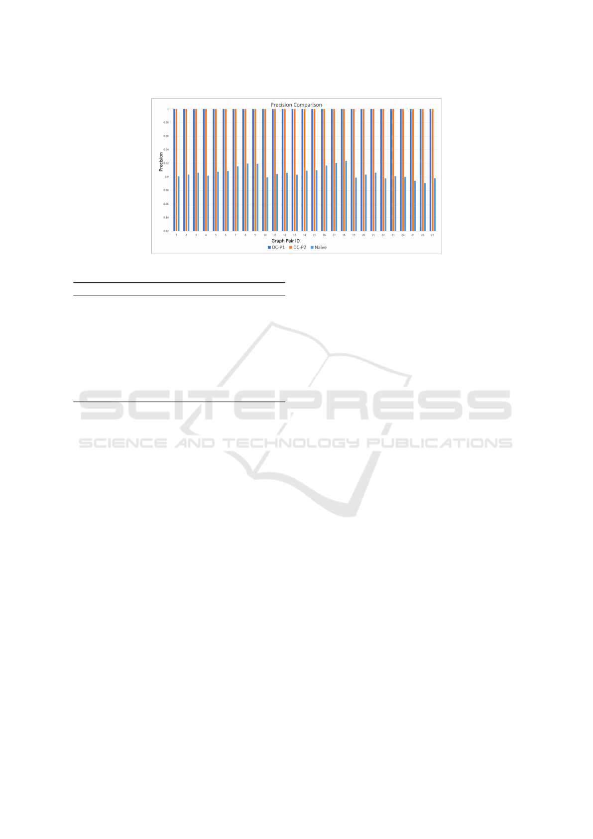
Figure 4: Precision Comparison for Synthetic Data Set 1 (Refer to Table 1).
Algorithm 2: Procedure for Θ using Heuristic DC-P1.
Require: DH
x
, avgDeg
x
, DH
y
, avgDeg
y
, NBD
x
,
NBD
y
, DH
xORy
←
/
0
1: avgEstDeg
xORy
← max(avgDeg
x
, avgDeg
y
)
2: for u ∈ DH
x
∪ DH
y
do
3: if |NBD
x
(u) ∪ NBD
y
(u)| >= avgEstDeg
xORy
then
4: DH
0
xORy
← DH
0
xORy
∪ u
5: end if
6: end for
Degree hubs and their values for each layer al-
low us to compute the higher bound of the average for
the aggregated graph. One-hop neighbor information
is used to reduce or eliminate false positives. How-
ever, as these are retained only for hubs, information
is still not complete. Even with this limited additional
information, as we will see in the experimental sec-
tion (Section 7.2), there is a significant improvement
in precision over the naive for all data sets. For the
synthetic data sets, we get a precision of 100% (Fig-
ure 4) and for the real-world data sets we get a mean
precision of 96% (Refer to Section 7.2, Figure 8).
6.2 Degree Centrality Heuristic
Precision(DC-P2)
Based on how the edges are distributed in the lay-
ers of a MLN, the actual average degree of the OR
composed ground truth, avgDeg
xORy
, of layers x and
y might differ from the estimated avgEstDeg
xORy
in
DC-P1. If the avgEstDeg
xORy
is substantially greater
than avgEstDeg
xORy
, then a lot of nodes will not be
included as a hub in the OR composed layer despite
having enough common neighbors across both layers
x and y. Similarly, if avgEstDeg
xORy
is smaller than
avgEstDeg
xORy
, a lot of false positives will be gener-
ated as hubs in the OR composed layer.
To better estimate the avgEstDeg
xORy
, we keep the
degree of each node from each layer as additional in-
formation during the Ψ step. This allows us to esti-
mate the individual degree of a node u in the OR com-
posed layer from its degree information in layer x and
layer y. If the degree of a node u in layer x is deg
x
(u)
and degree of the same node in layer y is deg
y
(u), then
estimated degree of node u in the OR composed layer,
estDeg
xORy
(u), is going to be max(deg
x
(u), deg
y
(u)).
Using the estimated degree estDeg
xORy
(u) of each
node u, we calculate the avgEstDeg
xORy
. The rest of
the steps of the algorithm are same as 2. As can be
seen in Figure 8, this heuristic slightly increases fur-
ther the precision value for some data sets.
7 EXPERIMENTAL ANALYSIS
7.1 Data Sets and Environment
The NetworkX (Hagberg et al., 2008) package is used
in our Python implementation. All experiments were
carried out on a single node SDSC Expanse (Towns
et al., 2014). Each node in the cluster runs the Cen-
tOS Linux operating system using an AMD EPYC
7742 CPU with 128 cores and 256GB of RAM hard-
ware. Both synthetic and real-world data sets were
used to evaluate the proposed methodologies. PaR-
MAT (Khorasani et al., 2015), a parallel version of the
popular graph generator RMAT (Chakrabarti et al.,
2004), which uses the Recursive-Matrix-based graph
generation technique, was used to create the synthetic
data sets.
We use PaRMAT to produce three sets of synthetic
data sets for each base graph for experimentation. Our
synthetic data set consists of 27 HoMLNs with two
layers, each with a different edge distribution. The
base graphs start with 100K vertices with 500K edges
KDIR 2022 - 14th International Conference on Knowledge Discovery and Information Retrieval
58
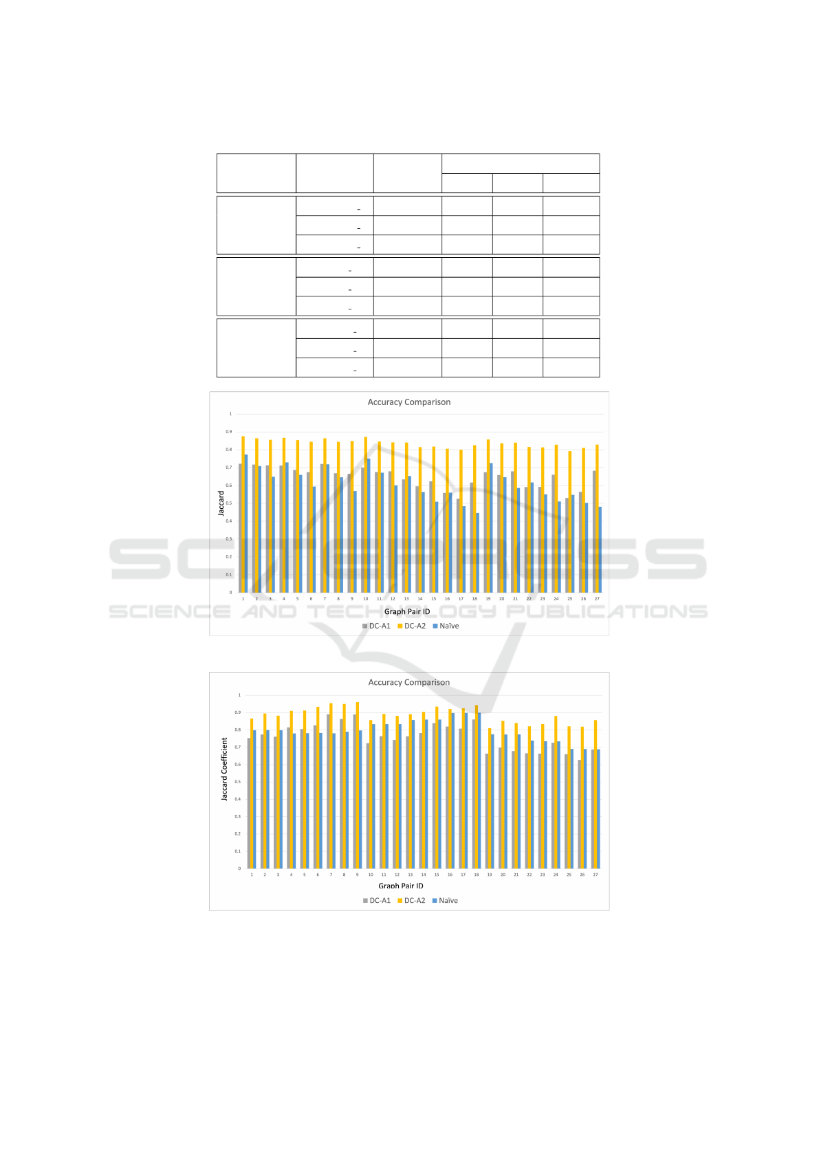
Table 2: Summary of Real World Data Set.
Base Graph
G
ID
Edge Dist. % #Edges
#Nodes, #Edges in Layers L1 L2 L1 OR L2
735KV, 2.6ME
amazon-2008 1 50,50 1306357 1304863 1958865
amazon-2008 2 70,30 1828100 784552 2063141
amazon-2008 3 90,10 2349969 261133 2376256
325KV, 1.7ME
cnr-2000 1 50,50 876444 876383 1314919
cnr-2000 2 70,30 1226781 525244 1384962
cnr-2000 3 90,10 1577646 175236 1595367
100KV, 1.5ME
uk-2007-05 1 50,50 759899 761252 1141215
uk-2007-05 2 70,30 1065435 455957 1202326
uk-2007-05 3 90,10 1369767 152167 1385013
Figure 5: Accuracy Comparison for Synthetic Data Set 2.
Figure 6: Accuracy Comparison for Synthetic Data Set 3.
and go up to 500K vertices and 10 million edges. In
the first synthetic data set (Table 1), both HoMLN lay-
ers have power-law degree distribution. In the second
synthetic data set (not shown, but similar to Table 1),
one layer (L1) follows power-law degree distribution
and the other one (L2) follows normal degree distri-
Degree Centrality Algorithms for Homogeneous Multilayer Networks
59
bution. In the final synthetic data set, both layers have
normal degree distribution (again not shown, but sim-
ilar to Table 1).
For each of the aforementioned data sets, three
edge distributions (70, 30; 60, 40; and 50, 50) for a
total of 81 HoMLNs with varied edge distributions,
number of nodes, and edges are used for experimen-
tation and validation of the proposed heuristics. Ta-
ble 1 shows the different 2-layer HoMLN used in our
data set used in our experiments which are part of the
synthetic data set 1. The synthetic data set 1 consists
of HoMLN where both the layers have the power-
law distribution of edges (L1: Power-law, L2: Power-
law). The other two data sets, synthetic data set 2 and
3 have a similar number of nodes and edges in each
layer but have (L1: Power-law, L2: Normal) and (L1:
Normal, L2: Normal) edge distribution.
For our real-world-like data set (shown in Ta-
ble 2), the network layers are generated from real-
world like monographs using a random number gen-
erator. The real-world-like graphs are generated us-
ing RMAT with parameters to mimic real-world graph
data sets as discussed in (Chakrabarti, 2005). As a re-
sult, the graphs are not single connected components
and neither are their ground truth graph.
7.2 Result Analysis and Discussion
In this section, we present our experimental results.
We have tested our proposed heuristics on large real-
world and synthetic data sets. As a measure of accu-
racy, we use the Jaccard coefficient and precision. We
compare the execution time of our heuristics against
the ground truth execution time as a measure of per-
formance. Figures 3, 5, and 6 show the Jaccard coef-
ficient for accuracy of the proposed heuristics-based
approaches DC-A1, DC-A2, and the naive approach
for the synthetic data set 1, data set 2, and data set
3 respectively. While calculating the Jaccard coeffi-
cient, we consider the nodes with equal to or higher
than the average degree value in the ground truth as
degree hubs. The heuristic DC-A2 performs the best
when the accuracy metric is the Jaccard coefficient.
It always shows higher accuracy than the naive ap-
proach. The heuristic DC-A1 performs better than
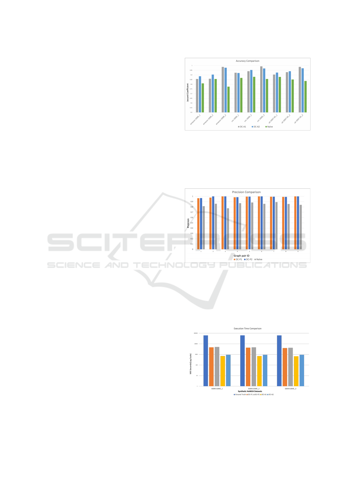
the naive approach in most cases. Figure 7 shows the
Jaccard coefficient for the proposed heuristics in real-
world data set (Boldi and Vigna, 2004). Both heuris-
tics DC-A1 and DC-A2 perform better than the naive
approach for all the HoMLN in the data set. Table 3
shows the mean accuracy and average percentage gain
in accuracy for the synthetic and real-world data sets.
For all data sets, DC-A2 outperforms the naive ap-
proach. The DC-A1 heuristic performs poorly when
Figure 7: Accuracy Comparison for Real World Data Set
(Refer to Table 2).
both layers have a normal distribution of edges, but
performs better than naive in other cases. One reason
for the low percentage gain compared to the naive ap-
proach is, that for Boolean OR aggregated HoMLN,
the naive approach itself has relatively high accuracy.
Figure 8: Precision Comparison for real world data set (Re-
fer to Table 2).
When precision is used as the measure of accu-
racy, DC-P1 and DC-P2 outperform DC-A1, DC-A2,
as well as the naive approach. For the synthetic data
sets, the precision of DC-P1 and DC-P2 is always
100% (Figure 4) and more than 96% for the real-
world data sets (Figure 8.)
Figure 9: Comparison of Execution Time of the Heuristics
against Execution Time of Ground Truth.
Figure 9 shows the comparison of the execution
time of our proposed solutions against the ground
KDIR 2022 - 14th International Conference on Knowledge Discovery and Information Retrieval
60
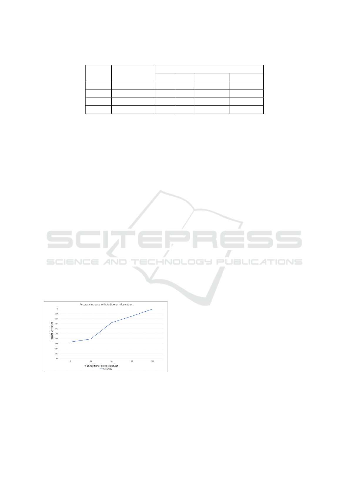
Table 3: Accuracy Improvement of DC-A1 and DC-A2 over Naive.
Data Set
Degree Distribution Mean Accuracy
L1, L2 DC-A1 DC-A2 DC-A1 vs. Naive DC-A2 vs. Naive
Synthetic-1 Power law, Power law 90.53% 96.01% +0.86% +6.96%
Synthetic-2 Power law, Normal 64.90% 83.74% +6.48% +37.38%
Synthetic-3 Normal, Normal 76.14% 88.72% -4.32% +11.47%
Real world Power law, Power law 93.11% 98.9% +10.03% +10.92%
truth time for 3 of the largest HoMLN of the syn-
thetic data set 1. The execution time of our approach
is calculated as maximum Ψ time of the layers + Θ
time. The ground truth time is computed as time re-
quired to aggregate layers into a single graph using
Boolean OR function + time required to find the de-
gree hubs of the aggregated graph.
As we can see from Figure 9, ground truth exe-
cution time is more than an order of magnitude as
compared to our proposed approaches in all cases
(plotted on log scale).
As previously mentioned in Section 3, it is a chal-
lenge to identify and keep the minimum amount of
information required in the network decoupling ap-
proach. Theoretically, as more information is kept,
the accuracy should go up. It is also affected by
the use of retained information based on intuition or
understanding of aggregation method used. For this
demonstration, we used a HoMLN consisting of 100K
nodes from the synthetic dataset 2 where the first layer
follows the power-law distribution and the second
layer follows the normal distribution. This HoMLN
was taken to minimize any similarity among the lay-
ers. The additional information kept is the one-hop
neighbors of the nodes in each layer.
Figure 10: Demonstration of increase in accuracy as more
information is kept in each layer for DC-A2.
In Figure 10 we show that as more information
is kept in each layer, the accuracy increases. If no
information is kept, we get the lowest accuracy. If we
keep one-hop neighbors of all the nodes, we get 100%
accuracy.
8 CONCLUSIONS AND FUTURE
WORK
In this paper, we proposed several heuristics-based al-
gorithms to compute degree hubs in a HoMLN di-
rectly using the decoupling approach. Some of the
heuristics (DC-A1 and DC-A2) achieve high accuracy
whereas others (DC-P1 and DC-P2) achieve a preci-
sion of 1. All proposed algorithms show more than
an order of magnitude improvement in efficiency
as compared to the traditional aggregation approach
used for ground truth. Our hypothesis with respect to
more information leading to higher accuracy is also
established. This heuristic-based approach has also
been applied for closeness centrality algorithms of ho-
mogeneous multilayer networks using the decoupling
approach with good results (Pavel et al., 2022).
Future work includes understanding the cascading
effects of accuracy and precision when more layers
are used. Also, how to identify and retain additional
information that can be used to improve the accuracy
of multiple layer centrality computation.
Acknowledgments: For this work, Drs. Sharma
Chakravarthy and Abhishek Santra were partly sup-
ported by NSF Grant CCF-1955798. Dr. Sharma
Chakravarthy was also partly supported by NSF Grant
CNS-2120393.
REFERENCES
DBLP Data Stats: https://dblp.uni-trier.de/statistics/
recordsindblp, Accessed: 24-May-2020.
Boldi, P. and Vigna, S. (2004). The WebGraph framework I:
Compression techaniques. In Proc. of the Thirteenth
International World Wide Web Conference (WWW
2004), pages 595–601, Manhattan, USA. ACM Press.
Boldi, P. and Vigna, S. (2014). Axioms for centrality. In-
ternet Mathematics, 10(3-4):222–262.
Brandes, U. (2001). A faster algorithm for betweenness
centrality. The Journal of Mathematical Sociology,
25(2):163–177.
Br
´
odka, P., Skibicki, K., Kazienko, P., and Musiał, K.
(2011). A degree centrality in multi-layered social net-
Degree Centrality Algorithms for Homogeneous Multilayer Networks
61

work. In 2011 International Conference on Compu-
tational Aspects of Social Networks (CASoN), pages
237–242.
Candeloro, L., Savini, L., and Conte, A. (2016). A
new weighted degree centrality measure: The ap-
plication in an animal disease epidemic. PloS one,
11(11):e0165781.
Chakrabarti, D. (2005). Tools for large graph mining.
Carnegie Mellon University.
Chakrabarti, D., Zhan, Y., and Faloutsos, C. (2004). R-mat:
A recursive model for graph mining. In Proceedings
of the 2004 SIAM International Conference on Data
Mining, pages 442–446. SIAM.
Cohen, E., Delling, D., Pajor, T., and Werneck, R. F. (2014).
Computing classic closeness centrality, at scale. In
Proceedings of the Second ACM Conference on On-
line Social Networks, COSN ’14, page 37–50, New
York, NY, USA. ACM.
De Domenico, M., Sol
´
e-Ribalta, A., Cozzo, E., Kivel
¨
a, M.,
Moreno, Y., Porter, M. A., G
´
omez, S., and Arenas,
A. (2013). Mathematical formulation of multilayer
networks. Physical Review X, 3(4):041022.
Everett, M. G. and Borgatti, S. P. (1999). The centrality
of groups and classes. The Journal of mathematical
sociology, 23(3):181–201.
Fortunato, S. and Castellano, C. (2009). Community struc-
ture in graphs. In Ency. of Complexity and Systems
Science, pages 1141–1163.
Gaye, I., Mendy, G., Ouya, S., Diop, I., and Seck, D.
(2016). Multi-diffusion degree centrality measure to
maximize the influence spread in the multilayer so-
cial networks. In International Conference on e-
Infrastructure and e-Services for Developing Coun-
tries, pages 53–65. Springer.
Hagberg, A., Swart, P., and S Chult, D. (2008). Explor-
ing network structure, dynamics, and function using
networkx. Technical report, Los Alamos National
Lab.(LANL), Los Alamos, NM (United States).
Khorasani, F., Gupta, R., and Bhuyan, L. N. (2015). Scal-
able simd-efficient graph processing on gpus. In
Proceedings of the 24th International Conference on
Parallel Architectures and Compilation Techniques,
PACT ’15, pages 39–50.
Kivel
¨
a, M., Arenas, A., Barthelemy, M., Gleeson, J. P.,
Moreno, Y., and Porter, M. A. (2014). Multilayer net-
works. Journal of Complex Networks, 2(3):203–271.
Kretschmer, H. and Kretschmer, T. (2007). A new central-
ity measure for social network analysis applicable to
bibliometric and webometric data. Collnet J. of and
Information Management, 1(1):1–7.
Liu, Y., Wei, B., Du, Y., Xiao, F., and Deng, Y. (2016). Iden-
tifying influential spreaders by weight degree central-
ity in complex networks. Chaos, Solitons & Fractals,
86:1–7.
Pavel, H. R., Santra, A., and Chakravarthy, S. (2022).
Closeness centrality algorithms for multilayer net-
works.
Pedroche, F., Romance, M., and Criado, R. (2016). A biplex
approach to pagerank centrality: From classic to mul-
tiplex networks. Chaos: An Interdisciplinary Journal
of Nonlinear Science, 26(6):065301.
Rachman, Z. A., Maharani, W., and Adiwijaya (2013). The
analysis and implementation of degree centrality in
weighted graph in social network analysis. In 2013
International Conference of Information and Commu-
nication Technology (ICoICT), pages 72–76.
Risselada, H., Verhoef, P. C., and Bijmolt, T. H. (2016). In-
dicators of opinion leadership in customer networks:
self-reports and degree centrality. Marketing Letters,
27(3):449–460.
Santra, A. and Bhowmick, S. (2017). Holistic analysis of
multi-source, multi-feature data: Modeling and com-
putation challenges. In Big Data Analytics - Fifth In-
ternational Conference, BDA 2017.
Santra, A., Bhowmick, S., and Chakravarthy, S. (2017a).
Efficient community re-creation in multilayer net-
works using boolean operations. In International Con-
ference on Computational Science, ICCS 2017, 12-14
June 2017, Zurich, Switzerland, pages 58–67.
Santra, A., Bhowmick, S., and Chakravarthy, S. (2017b).
Hubify: Efficient estimation of central entities across
multiplex layer compositions. In IEEE International
Conference on Data Mining Workshops.
Santra, A., Komar, K. S., Bhowmick, S., and Chakravarthy,
S. (2020). A new community definition for multilayer
networks and A novel approach for its efficient com-
putation. CoRR, abs/2004.09625.
Shi, Z. and Zhang, B. (2011). Fast network centrality anal-
ysis using gpus. BMC Bioinformatics, 12(1).
Sol
´
a, L., Romance, M., Criado, R., Flores, J., Garc
´
ıa del
Amo, A., and Boccaletti, S. (2013). Eigenvector
centrality of nodes in multiplex networks. Chaos:
An Interdisciplinary Journal of Nonlinear Science,
23(3):033131.
Srinivas, A. and Velusamy, R. L. (2015). Identification of
influential nodes from social networks based on en-
hanced degree centrality measure. In 2015 IEEE In-
ternational Advance Computing Conference (IACC),
pages 1179–1184.
Tang, X., Wang, J., Zhong, J., and Pan, Y. (2013). Pre-
dicting essential proteins based on weighted degree
centrality. IEEE/ACM Transactions on Computational
Biology and Bioinformatics, 11(2):407–418.
Towns, J., Cockerill, T., Dahan, M., Foster, I., Gaither, K.,
Grimshaw, A., Hazlewood, V., Lathrop, S., Lifka, D.,
Peterson, G. D., Roskies, R., Scott, J., and Wilkins-
Diehr, N. (2014). Xsede: Accelerating scientific
discovery. Computing in Science and Engineering,
16(05):62–74.
Uddin, S. and Hossain, L. (2011). Time scale degree cen-
trality: A time-variant approach to degree centrality
measures. In 2011 International Conference on Ad-
vances in Social Networks Analysis and Mining, pages
520–524. IEEE.
Wang, X., Hu, T., Yang, Q., Jiao, D., Yan, Y., and Liu, L.
(2021). Graph-theory based degree centrality com-
bined with machine learning algorithms can predict
response to treatment with antiepileptic medications
in children with epilepsy. Journal of Clinical Neuro-
science, 91:276–282.
Yang, Y., Dong, Y., and Chawla, N. V. (2014). Predicting
node degree centrality with the node prominence pro-
file. Scientific reports, 4(1):1–7.
KDIR 2022 - 14th International Conference on Knowledge Discovery and Information Retrieval
62
