
Spatial Simulation of the M
¨
uller-Lyer Illusion Genesis with
Convolutional Neural Networks
Anton N. Mamaev
a
and Ivan A. Gorbunov
b
Department of Psychology, St. Petersburg University, Makarova Embarkment 6, Saint Petersburg, Russian Federation
Keywords:
Optical Illusions, Depth Perception, Image-source Relationships, Computational Cognitive Science, Com-
puter Vision, Bayesian Statistics, Regression Problem.
Abstract:
The M
¨
uller-Lyer illusion is a well-known optical phenomenon with several competing explanations. In the
current study we reviewed the illusion in a convolutional neural network from a perspective of image-source
relationships in the process of visual functions development.
To recreate the effect of the illusion we proposed a novel method that lets us simulate the development of
visual functions in a controlled spatial environment from the state of ‘blank slate’ to effective spatial problem
solving. This process is designed to reflect the development of human visual system and enable us to determine
how depth perception can contribute to the appearance of the phenomenon.
We were able to successfully reproduce the effect of the classic M
¨
uller-Lyer in 30 independent convolutional
models and also get similar results with the variants of the illusion that are thought to be unrelated to spatial
perception. For the pairs of classic stimuli we conducted additional statistical analysis using both frequentist
and Bayesian methods. The methodological and empirical insights of this study may be helpful for subsequent
investigation of visual cognition and reconsideration of the image-source relationships in optical illusions.
1 INTRODUCTION
Since the introduction of the M
¨
uller-Lyer illusion
(Muller-Lyer, 1889) it received a number of theoreti-
cal explanations. Some of them view the phenomenon
as a result of adaptation to specific environments,
such as urban versus rural areas (Segall et al., 1963),
or the spatial perception constancy of size being mis-
applied to 2D images (Gregory, 1963) and others sug-
gest a physiological perspective and attribute the illu-
sion to the spatial summation of the postsynaptic po-
tentials in neurons in the receptive fields (Burns and
Pritchard, 1971).
Advances in the development of deep learning al-
gorithms made it possible to create complex mathe-
matical models with principles of operation similar
to natural neural networks of the human brain. This
opened up possibilities for new applications in the
field of cognitive sciences, such as modelling seman-
tic space (Gorbunov et al., 2019) and optical illusions
(Kubota et al., 2021), (Gomez-Villa et al., 2019). This
is also valid for convolutional models of the M
¨
uller-
a
https://orcid.org/0000-0002-2283-380X
b
https://orcid.org/0000-0002-7558-750X
Lyer illusion (Zeman et al., 2013), (Garc
´
ıa-Garibay
and de Lafuente, 2015). However, we believe that cur-
rent studies have not yet reached the limit of possible
approaches to optical illusion modelling.
One of the oversighted aspects is the possible us-
age of geometrically accurate computer graphics to
simulate spatial environments instead of 2D line art.
Although it was proven possible to reconstruct the
illusion without introducing image-source relation-
ships and 3D graphics, the discrepancies in human
and model performance forces one to acknowledge
the possibility of image-source relationships being
also a contributing factor (Zeman et al., 2013). We at-
tempt not only to reconstruct the effect of the M
¨
uller-
Figure 1: The M
¨
uller-Lyer illusion demonstration. While
the right line seems to be larger than the left one in ‘a’, it is
evident that they are equal in ‘b’.
284
Mamaev, A. and Gorbunov, I.
Spatial Simulation of the Müller-Lyer Illusion Genesis with Convolutional Neural Networks.
DOI: 10.5220/0011529100003332
In Proceedings of the 14th International Joint Conference on Computational Intelligence (IJCCI 2022), pages 284-291
ISBN: 978-989-758-611-8; ISSN: 2184-3236
Copyright © 2023 by SCITEPRESS – Science and Technology Publications, Lda. Under CC license (CC BY-NC-ND 4.0)

Lyer illusion in a neural network, but also to simulate
the genesis of the illusion from the point of view of
depth perception explanation.
In our study we revisit the image-source explana-
tion of the illusion by pre-training a model to solve a
regression problem of object height estimation in a 3D
environment before presenting a new but similar task
of estimating the length of the lines in the M
¨
uller-Lyer
illusion. By doing that we force the model to adapt to
a spatial environment, develop traits of depth percep-
tion, and transfer them to 2D stimuli. Moreover, the
model becomes capable of giving exact numerical es-
timations for all of the stimuli, in contrast to previous
studies that relied on the binary classification prob-
lem. This greatly enhances the differentiation of the
results, prevents random guessing, and facilitates sta-
tistical comparison with other models or human sub-
jects.
Compared to our preliminary study, we substan-
tially increased the sample of independent models
and validation images, performed a thorough quan-
titative analysis with Bayesian and frequentist statis-
tical methods, introduced new types of stimuli, and
broadened the theoretical scope of the research (Ma-
maev and Gorbunov, 2021).
Apart from investigating the causes of the M
¨
uller-
Lyer illusion and introducing unique methodology
that can be important for the advancement of com-
putational cognitive sciences, the study also can be
valuable from an industrial standpoint. Data set gen-
eration software can be used to pre-train computer vi-
sion models, and convolutional models such as the
one presented in this paper can be used as a measure-
ment tool. Finally, the susceptibility of convolutional
neural networks to optical illusions should be noted in
the development of models aimed for precision.
In the paper we will first review the specifications
of the neural model and the data sets, then present the
results of the statistical analysis and finally general-
ize the findings, provide our interpretation and sug-
gest the prospects for further studies.
2 MATERIALS AND METHODS
2.1 Data Sets
The model input data was divided into three separate
data sets:
1. Training data set (n = 500)
2. Validation data set (n = 100)
3. Testing data set (n = 12)
Images of the training data set were used to fit the
model. The validation data set has been excluded
from fitting and was used later to assess the model’s
accuracy on the new data. Both data sets were ren-
dered from a virtual 3D environment and contained
equivalent images. Each image depicted an internal
or external view on a cuboid mesh with a resemblance
to the geometry of a building or a room.
The training and validation data sets had target
values designated for every image in the array, as
shown in Figure 2. As the target values were the ob-
ject height values extracted directly from the image
source, the testing data set consisted only of input im-
ages.
Figure 2: Training and validation images with target values.
The testing images were conventional and uncon-
ventional variants of the M
¨
uller-Lyer illusion stimuli.
Original M
¨
uller-Lyer stimuli have arrows on the ends
of the lines that point either inside, towards the line
or outside, from the line. According to the illusion,
the ‘in’ lines are expected to be seen bigger than ‘out’
lines. Similarly, we also classified the variant stim-
uli with arrows replaced with other shapes as ‘in’ or
‘out’ depending on whether they are seen as larger or
smaller. All test stimuli are presented in Figure 3.
Figure 3: Testing data set stimuli pairs: a. narrow original;
b. wide original; c-e. variants from literature: d. (Hatwell,
1960), e. (Parker and Newbigging, 1963), c. Hatwell,
halved; f. our variant.
The virtual 3D environment was created with the
open source Godot 3.3.3 game engine. The scene
shown in Figure 4 included two cuboid meshes with
a mutual edge and a camera positioned inside one of
the meshes and pointed towards the edge.
Spatial Simulation of the Müller-Lyer Illusion Genesis with Convolutional Neural Networks
285
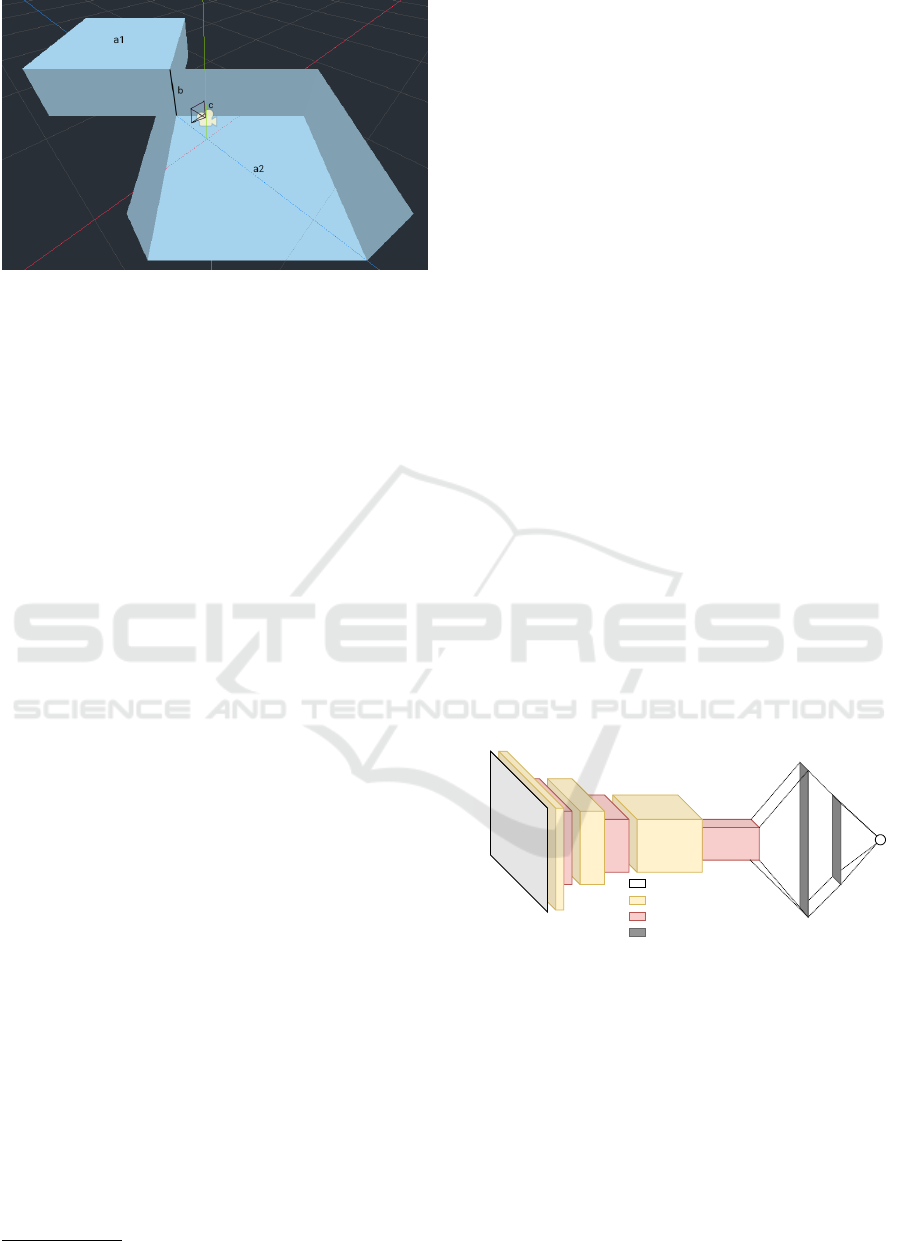
Figure 4: 3D environment overview: a1–2. object meshes;
b. mutual edge, length = target value; c: camera.
Several spatial parameters were randomly altered
for every picture taken by the camera in given ranges:
• Mesh heights (2.1,4.2),
• Camera distance (0,5),
• Camera y-axis rotation (−25,25),
• Mesh y-axis rotation (35,55).
The ranges were limited to selected values to ensure
that the angle fits into the field of view of the camera.
The heights of the meshes, being also the lengths
of their mutual edge, were exported in the image
metadata and used as target values to fit the model.
Other parameters such as mesh rotation, camera dis-
tance and camera rotation were randomized to aug-
ment the training data set so the model is trained in a
dynamic environment. This is done to enhance model
validity, as the model is forced to educe the laws of
spatial geometry to solve the problem from different
positions. It is also necessary to prevent overfitting, as
using highly similar data can render the model inca-
pable of generalizing on new data, making it impossi-
ble to estimate the illusion stimuli. The target values
are also necessary to be randomized, as the model is
expected to give a precise estimation for a picture with
an object of any given height.
The script used to generate batches of images with
randomized spatial parameters written in GDScript
1
is given below.
for i in range(n): #Generate n images
height = rand_range(2.1,4.2) #Mesh height
$Interior.mesh.size.y = height
$Exterior.mesh.size.y = height
if rand_rot == true: #Mesh rotation
rot = rand_range(35,55)
$Interior.rotation_degrees.y = rot
$Exterior.rotation_degrees.y = rot
if rand_dst == true: #Camera distance
1
Python-inspired scripting language of Godot
$Camera.translation.z =
rand_range(0,5)
if rand_angle == true: #Camera rotation
$Camera.rotation_degrees.y =
rand_range(-25,25)
if armed == true: #Toggle screenshots
image = get_viewport().get_texture()
.get_data()
image.flip_y()
image.save_png("../screenshots/"
+str(height)+".png")
print(str(i+1),". ",str(height)) #Log
2.2 Neural Network Architecture
The convolutional neural network was initially de-
veloped and tested on the limited datasets as part
of the previous stage of our research (Mamaev and
Gorbunov, 2021). It was designed and fitted with
Keras and Tensorflow frameworks for Python 3 in the
Google Colaboratory environment and followed a tra-
ditional architecture for its class, as shown in Figure
5. The shape of the input layer matched the grayscale
input images that were converted to 200×200×1 ma-
trices. The convolutional and max-pooling layers al-
ternated until the third max-pooling layer, after which
the data got flattened and transferred to the fully con-
nected layers. Except the output, all of the layers were
activated with the ReLU function.
Input/Output
Convolutional
Max Pooling
Fully connected
Conv1
32 3×3
Conv2
64 3×3
Conv3
128 3×3
MP3
2×2
MP2
2×2
MP1
2×2
FC1
n=1024
FC2
n=512
Input
200×200
Output
n=1
Figure 5: Convolutional neural network architecture
overview.
In contrast to typical convolutional neural net-
work architectures used for classification, our model
was initially designed to solve the regression prob-
lem and was converging on a single linear-activated
output neuron. Accordingly, the loss between the es-
timate and the real target value was calculated using
the mean squared error (eq. 1) function and the adap-
tive moment estimation function (Adam) was used as
a loss optimiser.
NCTA 2022 - 14th International Conference on Neural Computation Theory and Applications
286

MSE =
1
n
n
∑
i=1
(y
i
− ˆy
i
)
2
(1)
The image datasets, Godot project file of the-
dataset generator, the Jupyter notebook with Keras
source code and the final fitted model mentioned at
this section are available at Open Science Framework
(Mamaev, 2022).
2.3 Statistical Analysis
To determine the factors and the extent of the illu-
sion’s effect, we fitted a total of 30 independent mod-
els with the same training data set and made estima-
tions for the classic M
¨
uller-Lyer stimuli, classic stim-
uli with wide arrowheads, and four types of illusion
variants. Then we conducted both Bayesian and fre-
quentist statistical analyses represented by Markov
chain Monte Carlo (MCMC), Bayes Factor, Leave-
One-Out Cross-Validation (LOO), Watanabe-Akaike
Information Criterion (WAIC) and repeated measures
Analysis of Variance (ANOVA) respectively for the
estimations of narrow and wide classic stimuli.
As the results were obtained from a non-linear
model, the normality of the distribution could have
been substantially disrupted. This calls for statisti-
cal methods that would be more suitable for the as-
sessment of the deep neural networks. One of such
methods is Bayesian inference. Using MCMC algo-
rithms, we fitted four linear models that explain the
estimated values with the parameters of endpoint ar-
rows, the mean estimated line length and an indepen-
dent variable. The models corresponded to the hy-
potheses about the contribution of the arrowheads’
width and direction factors to the estimation results:
Model 1. Null model, arrowheads do not affect the
estimation:
Y = M
i
+ B
0
+ Err (2)
Model 2. In-Out model, the direction of the arrow-
heads affects the estimation:
Y = M
i
+ B
0
+ B
1
· X
in/out
+ Err (3)
Model 3. Narrow-Wide model, the width of the ar-
rowheads affects the estimation:
Y = M
i
+ B
0
+ B
2
· X
nrw/wd
+ Err (4)
Model 4. Full model, both the width and the direc-
tion of the arrowheads affect the estimation:
Y = M
i
+ B
0
+ B
1
· X
in/out
+ B
2
· X
nrw/wd
+ Err (5)
where:
Y : is the estimation made by the model
M
i
: is the mean of all estimations made by model i
B
0
: is the independent variable
B
1
: is the regression coefficient of In-Out factor (eq.
3 and 5)
B
2
: is the regression coefficient of the width factor
(eq. 4 and 5)
X
in/out
=
(
0, Inward arrows
1, Outward arrows
(eq. 3 and 5)
X
nrw/wd
=
(
0, Narrow arrows
1, Wide arrows
(eq. 4 and 5)
Err: is the model error
The models were fitted using PyMC3 and visual-
ized using Matplotlib and Arviz libraries for Python
3. An example of the source code is given below:
dev=numpy.std(Dependent)
with pymc3.Model() as Regr2Model:
#Define variables
b0=pymc3.Normal(’B0’,0,sd=dev*2)
b1=pymc3.Normal(’B1’,0,sd=dev*2
b2=pymc3.Normal(’B2’,0,sd=dev*2)
RegrError=pm.HalfCauchy(’Err’,
beta=10, testval=1.)
#Define likelihood
likelihood = pymc3.Normal(’Y’,
mu=MeanNet + b0
+ b1*Predictor1 + b2*Predictor2,
sd=RegrError, observed=Dependent)
#Trace posterior probability
Regr2FTrace = pymc3.sample(6000,
cores=3, tune=200)
Predictor 1 and 2 arrays represent the factors that
affect the values of the Dependent array.
3 RESULTS
3.1 Model Validation
After around 25-30 fitting epochs the neural network
loss was dropping lower than < 0.001. To evaluate
model’s generalization and accuracy on a new data
set we made estimations on the hold-out validation
data set of 100 images similar to the training data set.
Spatial Simulation of the Müller-Lyer Illusion Genesis with Convolutional Neural Networks
287
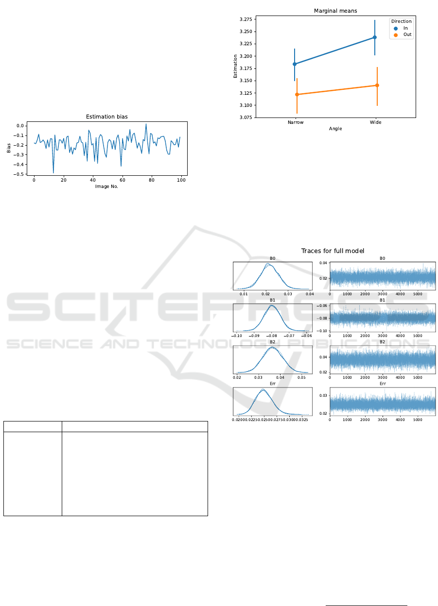
Figure 6 shows the bias between the model estima-
tions given for each image and the ground truth. The
values are close to zero, with the biggest peaks be-
ing ≤ ±0.5. The probable cause for the larger bias
in some images of the data set is the random nature
of the 3D scene. It is possible that some of the im-
ages lacked the visual features necessary for a precise
estimation because of an unfortunate camera-object
positioning.
Figure 6: Bias between the estimations and the ground truth
in the validation data set.
¯
X = −0.181,σ = 0.083.
¯
X: mean,
σ: std. deviation.
3.2 ANOVA
For an initial analysis, we used ANOVA with repeated
measures. The repeated measures were the estima-
tions given by 30 models for the same four M
¨
uller-
Lyer illusion stimuli. Details of the results are given
in Table 1. We have discovered a significant effect of
both the direction and the width of the arrowheads on
the variance of the estimates given by the model. The
directional factor η
2
= 0.822 influences the estima-
tions stronger than the width η
2
= 0.728. Together,
they also produce a smaller effect η
2
= 0.633.
Table 1: Detailed ANOVA results. SS: sum of squares, df:
degrees of freedom, MS: mean squares, F: F ratio.
SS df MS F
Intercept 1206.74 1 1206.74 32151.95
Error 1.088 29 0.038
N-W 0.04 1 0.040 77.74
Error 0.015 29 0.001
In-Out 0.191 1 0.191 135.06
Error 0.041 29 0.001
N-W×In-Out 0.010 1 0.010 49.96
Error 0.006 29 0.000
As shown in Figure 7, the lines with the arrow-
heads pointing inside are estimated to be longer than
those with the arrowheads pointing outside, accord-
ing to the principles of the M
¨
uller-Lyer illusion in hu-
mans. In addition, stimuli with wider arrows show a
greater divergence.
Figure 7: Marginal means for two factors: arrowheads di-
rection and angle. Vertical bars denote 95% confidence in-
tervals.
3.3 Bayesian Models
Figure 8 shows model traces and posterior plots made
with MCMC (Metropolis) algorithm. The similarities
of posterior distributions in all of the MCMC chains
is a favourable result in terms of the model fitness.
Figure 8: MCMC full model traces and posterior distribu-
tions.
As shown in Figure 9, the only parameter that is
not significantly different from zero is the indepen-
dent variable B
0
of the Null hypothesis model. Other
parameters are significantly divergent from zero with
94% highest density intervals.
The model error is at maximum in the Null hy-
pothesis model and at minimum in the Full model.
The In-Out model also has low error. This, again,
speaks in favour of the Full and In-Out models.
For further model comparison we used Bayes fac-
tor, WAIC and LOO:
BF(M
0
/M
Alt
) =
exp(
∑
log(P
0
(B|A))
exp(
∑
log(P
Alt
(B|A))
(6)
NCTA 2022 - 14th International Conference on Neural Computation Theory and Applications
288

Table 2: Specifications of the MCMC models.
¯
X: mean, σ: standard deviation, HDI: highest density intervals, ESS: effective
sample size,
ˆ
R: Gelman-Rubin convergence statistic.
Model Parameter
¯
X σ HDI 3% HDI 97% ESS (bulk) ESS (trial)
ˆ
R
Null B0 -0.000 0.005 -0.009 0.009 9201 7616 1
Null Err 0.051 0.003 0.044 0.067 7753 8702 1
In-Out B0 0.040 0.004 0.032 0.047 6863 8892 1
In-Out B1 -0.080 0.006 -0.090 -0.069 5021 6496 1
In-Out Err 0.031 0.002 0.027 0.035 9991 9487 1
N-W B0 -0.018 0.006 -0.030 -0.007 2981 6009 1
N-W B1 0.037 0.009 0.021 0.054 5822 8254 1
N-W Err 0.048 0.003 0.042 0.054 12445 11408 1
Full B0 0.021 0.004 0.014 0.029 6015 7011 1
Full B1 -0.080 0.005 -0.088 -0.071 10192 10726 1
Full B2 0.037 0.005 0.028 0.045 5608 5301 1
Full Err 0.025 0.002 0.022 0.028 11296 10509 1
Figure 9: Overall comparison of the calculated model pa-
rameters.
WAIC = −2
n
∑
i=1
log
1
S
S
∑
s=1
p(y
i
|θ
s
)
!
+
+
n
∑
i=1
S
∑
s=1
log p(y
i
|θ
s
)
!
(7)
el pd
LOO
=
n
∑
i=1
log(p(y
i
|y
−i
)) (8)
Table 3 illustrates the comparison between mod-
els with Bayes factor. The two-factor Full model
(3 · 10
37
) was chosen as the most probable, while the
In-Out (6.8 · 10
25
) and the Narrow-Wide (6.5 · 10
3
)
models were the second and the third respectively.
The scores were given relative to the least probable
Null model.
Comparison with the LOO method confirms the
Full model as the most probable. Small deviations in-
dicated in Figure 10 signify valid differences in the
models’ probabilities. Detailed results are shown in
Table 4. The WAIC results were similar but were not
Table 3: Bayes Factor model comparison.
Full In-Out Nrw-Wd Null
Full 1 2.3· 10
−12
2.2 ·10
−34
3.3 ·10
−38
I-O 4.4 ·10
11
1 9.7 · 10
−23
1.5 ·10
−26
N-W 4.6 · 10
33
1 ·10
22
1 1.5 ·10
−4
Null 3 ·10
37
6.8 ·10
25
6.5 ·10
3
1
plotted due to the warnings raised for two of the mod-
els.
Figure 10: Leave-One-Out Cross-Validation.
3.4 Illusion Variants
We used all of the 30 models used in the statistical
analysis to test them on the unconventional M
¨
uller-
Lyer illusion stimuli. Figure 11 illustrates the differ-
ences between the length estimations of ‘in’ and ‘out’
categories in each pair. The letters in the legend cor-
respond to images in Figure 3 for quick reference. As
there are no negative values the lines from the ‘in’ cat-
egory were estimated to be larger than from ‘out’ cat-
egory every single time across 30 models. The most
dramatic differences are found in pairs ‘d’ and ‘e’: in
those pairs, the line ended with either a square or a
circle. The smallest differences are in ‘c’ category:
the lines with square halves at the ends. Classic stim-
Spatial Simulation of the Müller-Lyer Illusion Genesis with Convolutional Neural Networks
289
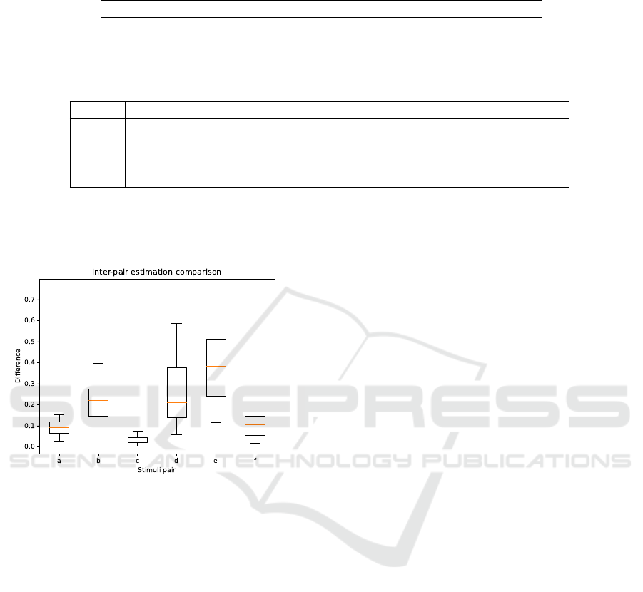
Table 4: Detailed LOO and WAIC model comparison report. pLOO, pWAIC: effective number of parameters, ∆LOO, ∆WAIC:
difference from the best-fitting model, SE: standard error, ∆SE: standard error of criterion’s difference from the best model.
Model Rank LOO pLOO ∆LOO Weight SE ∆SE
Full 0 270.70 4.67 0 9.89
−1
10.5 0
In-Out 1 245.21 3.31 25.49 1.14
−2
9.33 5.85
N-W 2 194.34 2.72 76.36 2.01
−12
6.86 6.4
Null 3 186.66 1.98 84.04 0 7.69 7.016029
Model Rank WAIC pWAIC ∆WAIC Weight SE ∆SE Warning
Full 0 270.73 4.64 0 9.89
−1
10.48 0 True
In-Out 1 245.22 3.3 25.51 1.11
−2
9.32 5.85 True
N-W 2 194.35 2.71 76.39 0 6.86 6.38 False
Null 3 186.66 1.98 84.07 1.23
−11
7.69 7.01 False
uli ‘a’ and our version ‘f’ showed comparable results
even though the new stimuli is highly different from
other M
¨
uller-Lyer illusion variations.
Figure 11: Estimated difference between ‘in’ and ‘out’
stimuli from the categories of the testing data set.
4 DISCUSSION
First of all, the model achieved high accuracy both
in the training and the validation data sets. With the
loss of < 0.001 and the estimate-truth divergence in
the validation set of 0.181 ± 0.083, the neural net-
work have been proven capable of solving spatial
tasks despite the randomized parameters of the envi-
ronment. This acknowledges the versatility of convo-
lutional neural networks and their capabilities in vi-
sual pattern recognition.
Secondly, the successful implementation of the
spatial simulation in the study of visual perception
opens a new opportunity for following studies. Opti-
cal illusions or other visual phenomena can be investi-
gated with geometrically accurate computer graphics
where maximum control over the environment is re-
quired.
Both Bayesian and frequentist statistical methods
that we used detected a significant effect of the direc-
tion and width of the arrows at the ends of the M
¨
uller-
Lyer illusion stimuli on the estimations made by the
model. The results of Bayesian model comparison
were unambiguous: all of the methods ranked the Full
model to be the most probable, followed by the In-
Out and Narrow-Wide models. The Null model was
ranked as the most unlikely. The consistency of the
ranking speaks in favour of its integrity. Such results
were not unexpected, as the original illusion is pri-
marily based on the direction of ending elements but
width also affects the estimations, perhaps depending
on the similarity of the wider arrows and the training
data set images.
The surprising discovery of the unconventional
M
¨
uller-Lyer stimuli being able to cause similar ef-
fects without depth cues not only in humans, but also
in a convolutional model fitted almost exclusively for
detection of depth cues requires thorough theoretical
review. However, in general, it is possible to pre-
sume that depth perception either coexists with an ad-
ditional independent cause of the illusion or both the
classic M
¨
uller-Lyer illusion and its non-perspective
variants take roots in the same phenomenon. Recep-
tive fields are good candidates, especially if we note
the similarities between them and the convolutional
filters. Convolutional neural networks are inspired by
the visual system’s anatomy and physiology, so they
are expected to have much in common. The weighted
spatial summation of retinal cells’ activation is re-
flected by the weights of filter matrix applied to the
values of the input image in an artificial neural net-
work, this way it is entirely possible to transfer the
neurophysiological explanation of the line ends being
subjectively shifted due to the context of additional
receptive field activation from the arrowheads to the
computational models. Yet the models are different
from nature as it is possible not only to directly study
single-cell activations or small groups of neurons but
also to study fully functional small-scale neural net-
NCTA 2022 - 14th International Conference on Neural Computation Theory and Applications
290

works (Lindsay, 2021). Those two approaches com-
plement the limitations of each other and broaden the
understanding of the phenomenon. We suppose both
the structure of visual system and the function of spa-
tial perception contribute to the appearance of the op-
tical illusions, however we are yet to understand the
interaction of those components while working with
various stimuli. A possible route we can take is to
study the inner states of the model: for example, the
filter weights and the feature maps of a neural model
are much easier to access than the internal states of
living neurons.
5 CONCLUSIONS
We have successfully recreated the M
¨
uller-Lyer illu-
sion in a convolutional neural network that was pre-
trained to estimate heights of the 3D object in a spatial
simulation. Transfer learning was successful and the
model was substantially biased when estimating the
illusion stimuli. We used Bayesian statistics to calcu-
late the impact of the image properties on the estima-
tions of the neural network and tested the model on
unconventional versions of the illusion.
Still, it is necessary to cover additional aspects of
the illusion in the next studies, such as the compar-
ison between the estimations of the neural network
and the mean estimations provided by humans for the
same images. Moreover, convolutional models may
be successfully used with other optical illusions, and
the study of the models’ inner states, as mentioned in
the previous section, can also be fruitful.
REFERENCES
Burns, B. D. and Pritchard, R. (1971). Geometrical illu-
sions and the response of neurones in the cat’s visual
cortex to angle patterns. The Journal of Physiology,
213(3):599–616.
Garc
´
ıa-Garibay, O. B. and de Lafuente, V. (2015). The
M
¨
uller-Lyer illusion as seen by an artificial neural net-
work. Frontiers in Computational Neuroscience, 9.
Gomez-Villa, A., Martin, A., Vazquez-Corral, J., and
Bertalmio, M. (2019). Convolutional Neural Net-
works Can Be Deceived by Visual Illusions. In
Proceedings of the IEEE/CVF Conference on Com-
puter Vision and Pattern Recognition (CVPR), pages
12309–12317.
Gorbunov, I., Pershin, I., Zainutdinov, M., and Koval, V.
(2019). Using the neural model of the person’s se-
mantic space to reveal the occurred with him events.
In 10th International Multi-Conference on Complex-
ity, Informatics and Cybernetics, IMCIC 2019, pages
164–165.
Gregory, R. L. (1963). Distortion of Visual Space as Inap-
propriate Constancy Scaling. Nature, 199(4894):678–
680. Number: 4894 Publisher: Nature Publishing
Group.
Hatwell, Y. (1960). Etude de quelques illusions
g
´
eom
´
etriques tactiles chez les aveugles. L’Ann
´
ee psy-
chologique, 60(1):11–27.
Kubota, Y., Hiyama, A., and Inami, M. (2021). A Ma-
chine Learning Model Perceiving Brightness Optical
Illusions: Quantitative Evaluation with Psychophys-
ical Data. In Augmented Humans Conference 2021,
AHs’21, pages 174–182, New York, NY, USA. As-
sociation for Computing Machinery. event-place:
Rovaniemi, Finland.
Lindsay, G. W. (2021). Convolutional Neural Networks
as a Model of the Visual System: Past, Present,
and Future. Journal of Cognitive Neuroscience,
33(10):2017–2031.
Mamaev, A. N. (2022). MLˆ2: the M
¨
uller-Lyer illusion
Machine Learning model.
Mamaev, A. N. and Gorbunov, I. A. (2021). The M
¨
uller-
Lyer illusion in CNN trained for 3D object height esti-
mation. In Neurotechnologies, pages 159–167. VVM,
St. Petersburg.
Muller-Lyer, F. (1889). Optische urteilstauschungen.
Archiv fur Anatomie und Physiologie, Physiologische
Abteilung, 2:263–270.
Parker, N. I. and Newbigging, P. L. (1963). Magnitude and
decrement of the M
¨
uller-Lyer illusion as a function of
pre-training. Canadian Journal of Psychology/Revue
canadienne de psychologie, 17(1):134–140.
Segall, M. H., Campbell, D. T., and Herskovits, M. J.
(1963). Cultural differences in the perception of ge-
ometric illusions. Science, 139(3556):769–771. Pub-
lisher: American Association for the Advancement of
Science.
Zeman, A., Obst, O., Brooks, K. R., and Rich, A. N.
(2013). The M
¨
uller-Lyer Illusion in a Computational
Model of Biological Object Recognition. PLoS ONE,
8(2):e56126.
Spatial Simulation of the Müller-Lyer Illusion Genesis with Convolutional Neural Networks
291
