
Suppression of Background Noise in Speech Signals with Artificial
Neural Networks, Exemplarily Applied to Keyboard Sounds
Leonard Fricke, Jurij Kuzmic and Igor Vatolkin
Department of Computer Science, TU Dortmund University, Otto-Hahn-Str. 14, Dortmund, Germany
Keywords: Artificial Neural Networks, Convolutional Neural Networks, Speech Enhancement, Noise Suppression,
Image Processing.
Abstract: The importance of remote voice communication has greatly increased during the COVID-19 pandemic. With
that comes the problem of degraded speech quality because of background noise. While there can be many
unwanted background sounds, this work focuses on dynamically suppressing keyboard sounds in speech
signals by utilizing artificial neural networks. Based on the Mel spectrograms as inputs, the neural networks
are trained to predict how much power of a frequency inside a time window has to be removed to suppress
the keyboard sound. For that goal, we have generated audio signals combined from samples of two publicly
available datasets with speaker and keyboard noise recordings. Additionally, we compare three network
architectures with different parameter settings as well as an open-source tool RNNoise. The results from the
experiments described in this paper show that artificial neural networks can be successfully applied to remove
complex background noise from speech signals.
1 INTRODUCTION AND
RELATED WORK
Recently, due to the COVID-19 pandemic, the role of
remote communication using audio and visual
transmission has significantly increased. However,
the quality of speech usually remains not perfect,
sometimes reasoned by limited speed of the network
connection, but also by various background noises:
keyboard sounds, another person speaking, street
noise, etc. The suppression of complex background
noise (like keyboard noise) is related to the topic of
speech enhancement. Traditional methods can handle
stationary background noise, for example white
noise. Commonly applied algorithms are the Wiener-
Filtering, the MMSE Estimator, or the Bayesian
Estimator (Loizou, 2013). They all provide different
techniques to estimate the components of the clean
short-time Fourier transform from a noisy input
signal. The techniques above all assume that the noise
signal is a stationary stochastic process that is
predicted and then removed from the signal. This is
not the case for keyboard typing sounds, because their
frequency curve is more complex. Furthermore,
different models of keyboards can sound entirely
different, and also the speed and intensity of typing
can vary significantly. For suppressing complex
background noise in speech signals, there exist
projects that utilize artificial neural networks. Krisp
(Krisp, 2021) and NVIDIA RTX Voice (NVIDIA,
2018) are both closed-source tools that work with
neural networks using GPU acceleration to suppress
keyboard noise in real time. These projects do not
offer details about what network architectures are
used and how they are trained. A similar open-source
project is RNNoise (Valin, 2021), which uses a small
recurrent neural network designed to run in embedded
systems with low computational power and no GPU
acceleration. Because of the low network complexity,
RNNoise is expected to underperform the neural
networks that will be proposed in this work.
However, it can be trained on a custom dataset which
allows for a direct comparison with the results of this
work.
In the following, we start with some backgrounds
on audio signal processing (Section 2). Then, the used
datasets and implemented network architectures are
presented in Section 3. The results of several studies
which compare the proposed networks and also apply
RNNoise are discussed in Section 4. The most
important findings are summarized in Section 5, and
several ideas for future work are proposed in Section
6.
Fricke, L., Kuzmic, J. and Vatolkin, I.
Suppression of Background Noise in Speech Signals with Artificial Neural Networks, Exemplarily Applied to Keyboard Sounds.
DOI: 10.5220/0011537400003332
In Proceedings of the 14th International Joint Conference on Computational Intelligence (IJCCI 2022), pages 367-374
ISBN: 978-989-758-611-8; ISSN: 2184-3236
Copyright © 2023 by SCITEPRESS – Science and Technology Publications, Lda. Under CC license (CC BY-NC-ND 4.0)
367

2 AUDIO SIGNAL PROCESSING
2.1 Signal Representation
In order to process a speech signal and separate it
from the background noise, a Short-Time Fourier
Transform (STFT) is applied. It converts the audio
signal into a representation where the power of
different frequencies over time can be displayed
(Loizou, 2013). A processed STFT spectrogram can
be easily inverted to output the original signal. In this
work, a STFT based on time frames of 512 samples
with a step size of 256 samples is used. With a sample
rate of 11025 Hz, this results in a window size of
approximately 23.22 ms. The spectrogram is then
projected to 128 Mel scale components, to take the
non-linearity in human frequency recognition
(Kathania et al., 2019) into account.
To allow for potential real time application, the
neural network only works on a small portion of the
input Mel spectrogram. The current time window is
selected together with the preceding 7 windows. This
leads to a network input size of 8 × 128 (see Figure
1). The network input is normalized using a
logarithmic transform and then rescaled to a range of
[0,1].
Figure 1: Example network input (8
× 128
).
2.2 Signal Separation
The neural network has to output the clean
spectrogram without background noise. While it is
possible to directly output the Mel spectrogram
values, we will use a mask to modify the magnitudes
in the spectrogram. The magnitude mask is defined
on the magnitudes of clean and noisy speech (Wang
and Chen, 2018):
𝑀𝑀
𝑡, 𝑘
|𝑆𝑡, 𝑘|
|𝑁𝑡, 𝑘|
(1)
S is defined as the spectrogram matrix of clean speech
and N is the matrix overlaid with the background
noise. The indices t and k are the time and frequency
containers in these matrices. This magnitude mask is
used as a target in the training process. After the
network predicts the mask, it can be element-wise
multiplied with the current time window of the input
spectrogram to recover the clean speech signal. The
values can be bounded between 0 and 1, because any
values 1 would only introduce an unnecessary
error. For
|
𝑁
𝑡, 𝑘
|
0, we can set this value to 1,
because there would be no background noise in that
container.
3 EXPERIMENT SETUP
3.1 Datasets
For the training process, a suitable dataset of both
speech and keyboard sound is needed. The speech
signals should come from different speakers and the
background noise should include multiple different
keyboard sounds to train a network with a good
general performance. The TIMIT Speech-Corpus
(Garofolo et al., 1993) was selected for the speech
data. It consists of 6300 spoken sentences by 630
different speakers of varying gender and origin.
Roughly 10% of the total speech data (624 sentences
by 24 speakers) were selected as the test set for the
final evaluation. From the remaining sentences, 80%
were used to train and 20% to validate the neural
networks. The speakers from the test set were not part
of the training set. For the background noise, a dataset
from DCASE 2016 (Lafay, Benetos and Lagrange,
2017) (Mesaros et al., 2018) was used. It contains
multiple types of background noise, in particular
typing sounds from 20 different keyboards. All audio
data was sampled at a rate of 11025 Hz. To generate
the noisy speech signals, every sentence in the TIMIT
dataset was overlaid with typing noise from a random
keyboard from the DCASE dataset. Every keyboard
noise was scaled with respect to loudness using
factors of 1.0, 1.5, 2.0, 2.5 and every sentence with
1.0, 1.5, 2.0, 2.5, 3.0, 3.5, 4.0. This further
increased the amount of available training data and
introduces a higher variance in volumes.
3.2 Neural Networks
We have tested three different network architectures.
First, a fully connected network consists of two
hidden layers with 500 units each with ReLU
activation and batch normalization. The output layer
has 128 units and sigmoid activation to ensure that the
mask values are between 0 and 1. This neural network
is denoted below as NN500.
Because the network input has a shape of 8 × 128,
a Convolutional Neural Network (CNN) might
perform better on two-dimensional data (Skansi,
2018). The used network has 4 convolutional layers
that each reduce the time dimensionality. In the
frequency dimension, a kernel size of 10 is combined
NCTA 2022 - 14th International Conference on Neural Computation Theory and Applications
368

with a stride of 1 in all layers. In the time dimension,
the kernel sizes are set to (8,4,2,2) and the strides to
(1,2,2,2). The kernel count is (32, 32, 16, 16) per
layer. Combined with zero-padding, this reduces the
shape to 1 × 128 during the convolutions. After the
convolution layers, the flattened activations are fed
through a fully connected hidden layer with ReLU
activation that is tested with different numbers of
neurons. The output layer again has 128 units and
sigmoid activation. The fully connected hidden layer
is tested with {128, 250, 500, 750} neurons. These
architectures are denoted as CNN128, ..., CNN750.
Third, a Redundant Convolutional Neural
Network (RCNN) is proposed, because it was shown
in (Park and Lee, 2017) that it can achieve
comparable results in speech enhancement with a
smaller network size. The network is built using 5
redundant blocks that each has 3 convolution layers
(Park and Lee, 2017). Each block has
(
18, 30, 8
)
kernels at a kernel size of
(
9, 5, 9
)
. With a stride of 1
and zero-padding, there is no dimension reduction
between the blocks. The redundant convolutions
reduce the time dimension of the input in the first
block and thus have significantly less parameters than
the CNNs. Just like in the traditional CNNs, the
flattened activations are fed through a fully connected
hidden layer with ReLU activation that is tested with
{
128, 250, 500
}
neurons. The magnitude mask is
output using a layer with 128 units and sigmoid
activation. The RCNN architectures are denoted as
RCNN128, ..., RCNN500. Additionally, we test a
RCNN without a fully connected hidden layer,
denoted as RCNN.
All neural networks are trained using an ADAM
Optimizer (Bock and Weiß, 2019) with a learning rate
of 0.0001 and a batch size of 128 for 100 epochs. For
the loss function, the mean squared error of the
magnitude masks is used.
4 EVALUATION OF
EXPERIMENTS
4.1 Initial Training
Table 1 presents the overview of several evaluation
measures estimated for the test set. Columns 2 and 3
show the Mean Squared Errors (MSE) for the
generated masks (Eq. 2) and the respective
spectrograms (Eq. 3). The best results with respect to
𝑀𝑆𝐸
and 𝑀𝑆𝐸
are achieved by CNN750. The
remaining CNN architectures all perform marginally
better than the redundant convolution networks.
RCNN250 reaches the lowest error out of the tested
RCNNs. To show the differences between the
examined network models, their output can be
visually compared.
𝑀𝑆𝐸
=
1
𝑇𝐾
𝑀𝑀
(
𝑡, 𝑘
)
−𝑀𝑀
(
𝑡, 𝑘
)
(2)
𝑀𝑆𝐸
=
1
𝑇𝐾
(|
𝑁
(
𝑡, 𝑘
)|
−|𝑆
(
𝑡, 𝑘
)
|
)
(3)
𝑀𝑀
represents the magnitude mask of the clean
target signal. In Figures 2 to 5, example Mel
spectrograms generated by the best and worst
network are displayed. Figure 2 presents the
spectrogram of the mixed signal, and Figure 3 the
target output (speech without keyboard noise). When
comparing the outputs to the target outputs, we can
see that the simple network in Figure 4 only partially
removes the keyboard noise. The best network so far,
CNN750 shows better visual results in Figure 5. In the
output spectrogram, there is only a little keyboard
sound left. Even though it is still hearable in the
signal, the volume of the typing noise has
significantly decreased.
Because even the best network in the initial
experiments did not fully remove the keyboard noise,
further investigation of the network error was
necessary. The assumption was used that the human
perception of errors in spectrograms is not symmetric.
As it was proposed in (Loizou, 2005), a positive error
(
|
𝑁
(
𝑡, 𝑘
)|
−𝑆(𝑡, 𝑘)| > 0) has a larger effect on
perception than a negative error (
|
𝑁
(
𝑡, 𝑘
)|
−
𝑆(𝑡, 𝑘)| < 0). A positive error means that there is
background noise remaining in the signal and a
negative error means that the speech signal has lost
power in that frequency container. To analyze these
errors, the metrics 𝑀𝑆𝐸
(positive error) and
𝑀𝑆𝐸
(negative error) are introduced:
𝑀𝑆𝐸
=
1
𝑇𝐾
max
{
0,
(|
𝑁
(
𝑡, 𝑘
)|
−
|
𝑆
(
𝑡, 𝑘
)|)
}
(4)
𝑀𝑆𝐸
=
1
𝑇𝐾
min
{
0,
(|
𝑁
(
𝑡, 𝑘
)|
−
|
𝑆
(
𝑡, 𝑘
)|)
}
(5)
Suppression of Background Noise in Speech Signals with Artificial Neural Networks, Exemplarily Applied to Keyboard Sounds
369
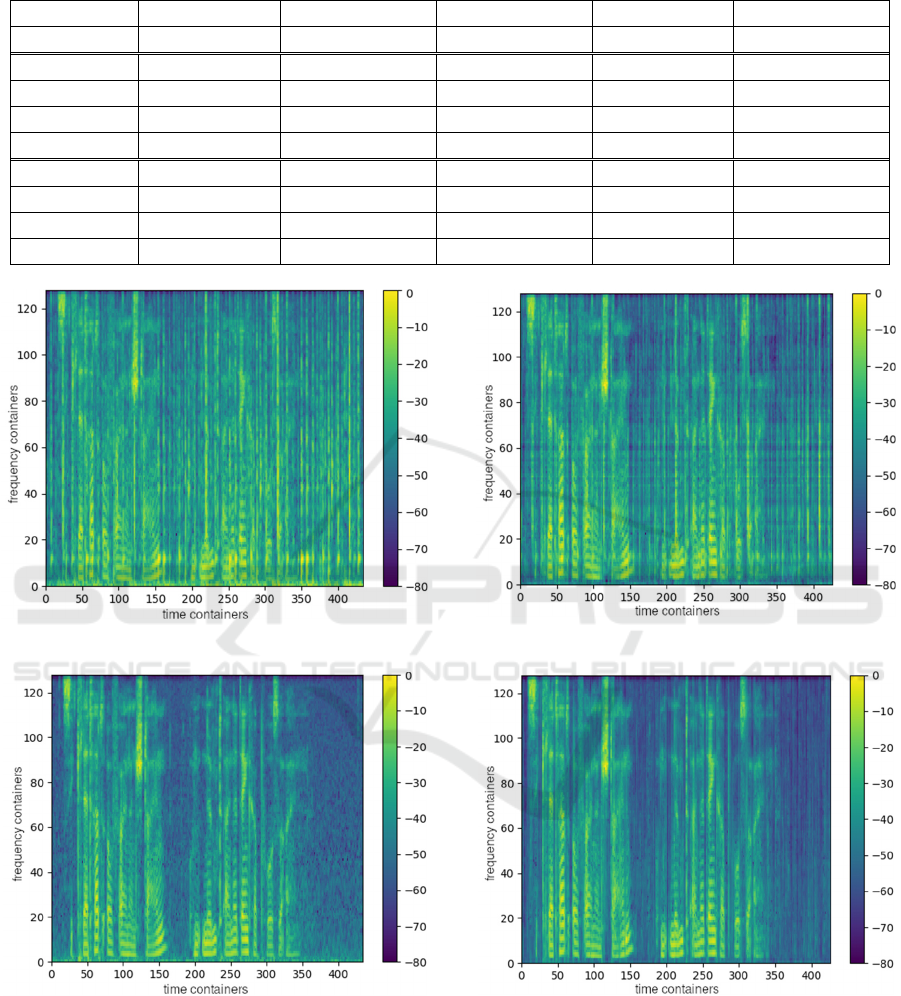
Table 1: Evaluation of different networks on the test set. The best values for CNNs and RCNNs are highlighted.
Network MSE
mask
MSE
spec
MSE
noise
MSE
speech
MIS
NN500 0.071 1.855 ‧ 10
−5
1.267 ‧ 10
−5
5.885 ‧ 10
−6
9.245 ‧ 10
−6
CNN128 0.031 7.039 ‧ 10
−6
2.076 ‧ 10
−6
4.963 ‧ 10
−6
3.539 ‧ 10
−6
CNN250 0.028 6.629 ‧ 10
−6
1.915 ‧ 10
−6
4.713 ‧ 10
−6
3.331 ‧ 10
−6
CNN500 0.026 6.127 ‧ 10
−6
1.745 ‧ 10
−6
4.382 ‧ 10
−6
3.078 ‧ 10
−6
CNN750 0.025 5.798 ‧ 10
−6
1.656 ‧ 10
−6
4.143 ‧ 10
−6
2.913 ‧ 10
−6
RCNN 0.080 1.830 ‧ 10
−5
1.129 ‧ 10
−5
7.014 ‧ 10
−6
9.146 ‧ 10
−6
RCNN128 0.045 1.324 ‧ 10
−5
8.040 ‧ 10
−6
5.201 ‧ 10
−6
6.595 ‧ 10
−6
RCNN250 0.033 7.316 ‧ 10
−6
2.707 ‧ 10
−6
4.609 ‧ 10
−6
3.669 ‧ 10
−6
RCNN500 0.035 9.242 ‧ 10
−6
2.926 ‧ 10
−6
6.315 ‧ 10
−6
4.646 ‧ 10
−6
Figure 2: Example input spectrogram.
Figure 3: Example target output spectrogram.
As listed in columns 4 and 5 in Table 1, these errors
show similar results as before. CNN750 is still the
best performing CNN network and RCNN250 is the
best RCNN network which is marginally worse than
the CNNs. For all neural networks, the 𝑀𝑆𝐸
is
lower than the 𝑀𝑆𝐸
.
Figure 4: Example output spectrogram of NN500.
Figure 5: Example output spectrogram of CNN500.
The different perceptual meaning of these errors
can also be expressed by another evaluation measure,
the modified Itakura-Saito Divergence (MIS)
(Loizou, 2005). It was designed to represent this
effect using an additional exponential term:
NCTA 2022 - 14th International Conference on Neural Computation Theory and Applications
370
𝑀𝐼𝑆 =
1
𝑇𝐾
exp
(|
𝑁
(
𝑡, 𝑘
)|
−
|
𝑆
(
𝑡, 𝑘
)|)
−
(|
𝑁
(
𝑡, 𝑘
)|
−
|
𝑆
(
𝑡, 𝑘
)|)
−1
(6)
Table 1, column 6 shows that the 𝑀𝐼𝑆 of the trained
network models validated on the test set also shows
similar results compared to other evaluation
measures.
4.2 Adapting the Loss Function
In the following, the different effects of 𝑀𝑆𝐸
and
𝑀𝑆𝐸
were applied to the loss function to further
improve the results. In Equation 7, the MSE of the
magnitude masks is separated and the positive part is
weighted with a hyperparameter α:
𝐿 =
1
𝐾
max 0, (𝑀𝑀
(
𝑘
)
−𝑀𝑀
(
𝑘
)
)
∙𝛼
min 0, (𝑀𝑀
(
𝑘
)
−𝑀𝑀
(
𝑘
)
)
(7)
Based on the preliminary experiments, the adapted
loss function was used with values 4.0 and 8.0 for α.
Besides the new loss, the neural networks were
trained using the same setup as before. In Table 2, the
evaluation measures for the networks trained with the
new loss function with α = 8.0 are shown. It can be
observed that the values for 𝑀𝑆𝐸
are much lower
than with the original loss function reported in Table
1. Now, CNN500 achieves the best error with respect
to 𝑀𝑆𝐸
. On the other hand, 𝑀𝑆𝐸
is higher
for all networks, which indicates a tradeoff in speech
quality. But because this error is less important for the
perceived speech quality (Loizou, 2005), the
decreased 𝑀𝑆𝐸
might have the advantage of
almost complete removal of the background noise.
The modified Itakura-Saito Divergence slightly
increases for most networks which can be explained
by the overall higher error 𝑀𝑆𝐸
. The network
CNN500 which had the lowest value of 𝑀𝑆𝐸
also
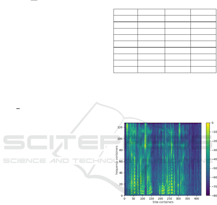
reaches the best value in 𝑀𝐼𝑆. The visualized
example output in Figure 6 shows the improvement
compared to the initial loss function. There is almost
no keyboard noise visible in the output spectrogram.
It is noticeable that the areas in the spectrogram where
no speech is present are displayed much darker.
Table 2: Evaluation measures estimated for the test set
using the adapted loss function (α = 8.0). The best values
are highlighted.
Network MSE
noise
MSE
speech
MIS
NN500 2.788 ‧ 10
−6
3.841 ‧ 10
−5
2.130 ‧ 10
−5
CNN128 4.140 ‧ 10
−7
1.149 ‧ 10
−5
6.017 · 10
−6
CNN250 3.675 ‧ 10
−7
1.102 ‧ 10
−5
5.758 · 10
−6
CNN500 2.594 ‧ 10
−7
1.164 ‧ 10
−5
2.164 · 10
−6
CNN750 3.123 ‧ 10
−7
9.723 ‧ 10
−6
5.072 · 10
−6
RCNN 1.050 ‧ 10
−6
1.021 ‧ 10
−5
5.686 · 10
−6
RCNN128 4.408 ‧ 10
−7
1.442 ‧ 10
−5
7.512 · 10
−6
RCNN250 6.649 ‧ 10
−7
1.079 ‧ 10
−5
5.784 · 10
−6
RCNN500 6.420 ‧ 10
−7
9.354 ‧ 10
−6
5.040 · 10
−6
As this is just normal noise from the recording, the
significant parts of the speech signal remain. The
newly trained networks remove that part from the
spectrogram, which increases the error of speech
𝑀𝑆𝐸
. Even though the error is increased, the
visualization shows that the speech signal is still
preserved in the output.
Figure 6: Example output spectrogram of CNN500 trained
with the adapted loss function (α = 8.0).
4.3 Combination of Different Noise
Types
In the experiments so far, the neural networks were
only trained to suppress keyboard noise. To test
whether the proposed network architectures can also
work on multiple background noise types, a new
training dataset was created. This dataset was
generated using the same procedure as described in
Section 3.1, but instead of keyboard noise, 20
different door knocking sounds from the DCASE
2016 (Lafay, Benetos and Lagrange, 2017) (Mesaros
et al., 2018) dataset were selected. The resulting door
Suppression of Background Noise in Speech Signals with Artificial Neural Networks, Exemplarily Applied to Keyboard Sounds
371
knock dataset has the same size as the keyboard
training, validation, and test sets together. They were
randomly mixed to create a combined dataset. In
these experiments, only the three traditional
convolutional neural networks were trained on the
combined training dataset using the adapted loss
function α = 8.0. In Table 3, the trained networks
are evaluated on the keyboard validation set and in
Table 4 on the door knock validation set.
Table 3: Evaluation measures of the combined networks
estimated for the test set for keyboard noise.
Network MSE
noise
MSE
speech
MIS
CNN128 4.986 ‧ 10
−7
1.177 ‧ 10
−5
6.202 ‧ 10
−5
CNN250 3.790 ‧ 10
−7
1.157 ‧ 10
−5
5.041 · 10
−6
CNN500 3.350 ‧ 10
−7
1.090 ‧ 10
−5
5.685 · 10
−6
Table 4: Evaluation measures of the combined networks
estimated for the test set for door knock noise.
Network MSE
noise
MSE
speech
MIS
CNN128 2.254 ‧ 10
−6
6.800 ‧ 10
−5
3.663 ‧ 10
−5
CNN250 1.402 ‧ 10
−6
6.729 ‧ 10
−5
3.581 · 10
−5
CNN500 1.382 ‧ 10
−6
6.188 ‧ 10
−5
3.297 · 10
−5
In general, it can be observed that the keyboard noise
has a lower error than door knocking. Compared to
the previous training on keyboard noise with the
adapted loss function, the 𝑀𝑆𝐸
slightly increases
while the 𝑀𝑆𝐸
slightly decreases. All in all, the
combination of two different noise types does work.
It delivers comparable validation errors while using
the same neural network for two different background
sounds.
4.4 Comparison with RNNoise
In a further experiment, we have compared the
previous results to the open-source software RNNoise
(Valin, 2021). RNNoise uses a smaller recurrent
neural network running on different features, as
explained in (Valin, 2018). The software comes with
a pre-trained network, but to get a better comparison
of the architectures, RNNoise was trained on the
dataset with keyboard noise from Section 3.1 using
the method from (Valin, 2018). The resulting network
was evaluated on the test set for keyboard noise and
compared to the network CNN500 trained with the
adapted loss function (α = 8.0). The evaluation
measures are listed in Table 5. Note that RNNoise
only consists of 88,007 parameters while the CNN500
has 1,149,992. RNNoise reaches higher errors than
the convolutional neural network in all measures. It
must be stated that RNNoise uses a much smaller
network which justifies the worse performance. A
noticeable result is that RNNoise has a significantly
lower 𝑀𝑆𝐸
compared to the other measures. The
error is smaller than the error of the networks that
were trained using the 𝑀𝑆𝐸 loss function in the initial
training.
Table 5: Evaluation measures of RNNoise and CNN500
(α = 8.0) estimated for the test set for keyboard noise.
RNNoise CNN500
MSE
spec
2.196 ‧ 10
−4
1.190 ‧ 10
−5
MSE
noise
9.154 ‧ 10
−7
2.594 · 10
−7
MSE
speech
2.187 ‧ 10
−4
1.164 · 10
−5
MIS 1.166 ‧ 10
−4
2.164 · 10
−6
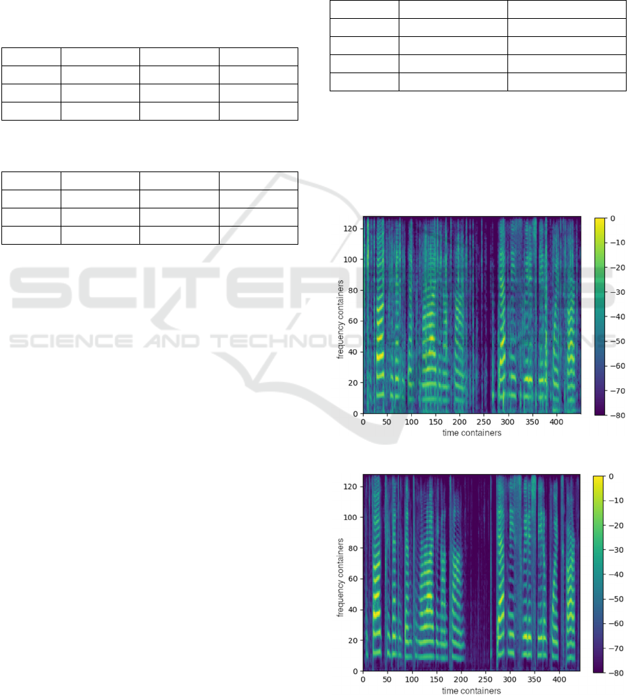
The results of RNNoise were also visually compared
to the network CNN500, as exemplarily shown in
Figures 7 and 8. RNNoise manages to only partially
remove the keyboard sound. The neural network from
this work can outperform RNNoise, as there is almost
no keyboard sound visible in the Mel spectrogram.
Figure 7: Example output spectrogram of RNNoise.
Figure 8: Example output spectrogram of CNN500 trained
with the adapted loss function (α = 8.0).
NCTA 2022 - 14th International Conference on Neural Computation Theory and Applications
372

5 CONCLUSIONS
In this work, keyboard sounds were dynamically
suppressed in speech signals using artificial neural
networks. The inputs to the networks were small time
frames of the Mel spectrograms, and the target was to
predict a magnitude mask that can remove the
background noise from the input signal. In the first
experiments, the background signal was only partially
suppressed and remained in the output signal at a
much lower volume. The best results were achieved
using convolutional neural networks.
The adaptation of the loss function, in order to
reach a better suppression of the keyboard noise, led
to a significantly better removal of the background
noise. Especially in the visual comparison of the
output spectrograms with the results from the initial
experiments, the improvement was recognized.
Further, we explored whether the proposed neural
networks can work on multiple different background
noise types. A combined dataset was created with
keyboard and door knocking sounds mixed together.
The networks trained on the combined training set
showed only marginally higher errors than the
previous experiments.
Finally, the results achieved in this work were
compared to the open-source tool RNNoise. It was
determined that the convolutional neural network
from the experiments outperforms RNNoise. This
might be justified because RNNoise uses a much
smaller network.
In conclusion, this topic is not new and has been
researched for some time. The problem in academic
research is that algorithms and procedures which are
already established in the commercial software are
not freely accessible. For this reason, own algorithms
and procedures have to be researched and developed
in the academic field. This paper presents a system for
removing complex background noises from speech
signals using the example of computer keyboard
noise. Thus, it is possible to develop a non-cost
software in a short time adapted to own background
noises. To assess the quality of our solution, further
experiments and different background noises are
necessary.
6 FUTURE WORK
Some of the network hyperparameters were not
varied in the experiments. It can be further
investigated whether the number of the Mel
frequency containers can be reduced without a
significant impact on the quality of the output. A
lower number of containers per time window would
also drastically decrease the network size and
computation time. Further, the network architectures
can be even automatically learned using neural
architecture search (Elsken, Metzen and Hutter,
2019). It is expected that the error values as well as
the network size can be decreased by systematically
exploring new architectures. Also, different loss
functions can be used. The adapted loss from this
work has to be tested with more fine-grained values
of α, but there might be more suitable loss functions.
For an application of such a system, more noise
types must be taken into account. It was shown that
two different types can be combined, but the training
data could be extended, for example, with fan noise,
baby screaming, or traffic sounds. When transferring
speech signals over the Internet in real time, a packet
loss can occur. The proposed system could be trained
to predict the missing time windows from the
previous ones. As an extension of the work, run time
measurements of the presented method can be carried
out. Thus, various comparisons can be made with
other NN-based or traditional methods.
REFERENCES
Bock, S., Weiß, M., 2019. A Proof of Local Convergence
for the Adam Optimizer. International Joint Conference
on Neural Networks (IJCNN), ISBN: 978-1-7281-
1985-4, pp. 1-8.
Elsken, T., Metzen, J. H., Hutter, F., 2019. Neural
Architecture Search: A Survey. Journal on Machine
Learning Research, vol. 20, pp. 55:1-55:21.
Garofolo, J., Lamel, L., Fisher, W., Fiscus, J., Pallett, D.,
Dahlgren, N., 1993. TIMIT Acoustic Phonetic
Continuous Speech Corpus. Linguistic Data Consortium.
Krisp, 2021. HD Voice with Echo and Noise Cancellation.
Krisp.ai. [online]. Available at: https://krisp.ai/.
Accessed: 22/12/2021.
Kathania, H., Shahnawazuddin, S., Ahmad, W., Adiga, N.,
2019. On the Role of Linear, Mel and Inverse-Mel
Filterbank in the Context of Automatic Speech
Recognition. National Conference on Communications
(NCC), ISBN 978-3-658-23751-6, pp. 1-5.
Lafay, G., Benetos, E., Lagrange, M., 2017. Sound event
detection in synthetic audio: Analysis of the DCASE
2016 task results. IEEE Workshop on Applications of
Signal Processing to Audio and Acoustics (WASPAA),
ISBN: 978-1-5386-1632-1, pp. 11-15.
Loizou, P., 2013. Speech Enhancement: Theory and
Practice. Second Edition. CRC Press, 2013.
Loizou, P., 2005. Speech Enhancement Based on
Perceptually Motivated Bayesian Estimators of the
Magnitude Spectrum. IEEE/ACM Transactions on
Suppression of Background Noise in Speech Signals with Artificial Neural Networks, Exemplarily Applied to Keyboard Sounds
373

Audio, Speech, and Language Processing, ISSN: 1063-
6676, vol. 13, no. 5, pp. 857-869.
Mesaros, A., Heittola, T., Benetos, E., Foster, P., Lagrange,
M., Virtanen, T., Plumbley, M., 2018. Detection and
Classification of Acoustic Scenes and Events: Outcome
of the DCASE 2016 Challenge. IEEE/ACM
Transactions on Audio, Speech, and Language
Processing, ISSN: 2329-9290, vol. 26, no. 2, pp. 379-
393.
NVIDIA, 2018. NVIDIA RTX Voice. Nvidia.com. [online].
Available at: https://developer.nvidia.com/blog/nvidia-
real-time-noise-suppression-deep-learning/. Accessed
22.12.2021].
Park, S., Lee, J., 2017. A Fully Convolutional Neural
Network for Speech Enhancement. Interspeech, pp.
1993 - 1997.
Skansi, S., 2018. Introduction to Deep Learning. Springer,
2018.
Valin, J., 2021. RNNoise. Gitlab.org. [online]. Available at:
https://gitlab.xiph.org/xiph/rnnoise/. Accessed: 22/12/
2021.
Valin, J., 2018. A Hybrid DSP/Deep Learning Approach to
Real-Time Full-Band Speech Enhancement. IEEE 20th
International Workshop on Multimedia Signal
Processing (MMSP), ISBN: 978-1-5386-6070-6.
Wang, D., Chen, J., 2018. Supervised Speech Separation
based on Deep Learning: An Overview. IEEE/ACM
Transactions on Audio, Speech, and Language
Processing, ISSN: 2329-9290, vol. 26, no. 10, pp. 1702-
1726.
NCTA 2022 - 14th International Conference on Neural Computation Theory and Applications
374
