
A Novel Approach towards Gap Filling of High-Frequency Radar
Time-series Data
Anne-Marie Camilleri
1
, Joel Azzopardi
1
and Adam Gauci
2
1
Department of Artificial Intelligence, Faculty of ICT, University of Malta, Msida, Malta
2
Department of Geosciences, Faculty of Sciences, University of Malta, Msida, Malta
Keywords:
Time-series Analysis, Deep Learning, Machine Learning, Gap Filling, High Frequency Radar.
Abstract:
The real-time monitoring of the coastal and marine environment is vital for various reasons including oil spill
detection and maritime security amongst others. Systems such as High Frequency Radar (HFR) networks
are able to record sea surface currents in real-time. Unfortunately, such systems can suffer from malfunc-
tions caused by extreme weather conditions or frequency interference, thus leading to a degradation in the
monitoring system coverage. This results in sporadic gaps within the observation datasets. To counter this
problem, the use of deep learning techniques has been investigated to perform gap-filling of the HFR data.
Additional features such as remotely sensed wind data were also considered to try enhance the prediction ac-
curacy of these models. Furthermore, look-back values between 3 and 24 hours were investigated to uncover
the minimal amount of historical data required to make accurate predictions. Finally, drift in the data was also
analysed, determining how often these model architectures might require re-training to keep them valid for
predicting future data.
1 INTRODUCTION
The growth of the blue economy and maritime opera-
tions, and the importance given to sustainable oceans
has rendered the availability of real-time oceano-
graphic observation and forecast data to be crucial in
this day and age. Such data can be used in various
applications such as oil spill response, maritime se-
curity, and monitoring of the coast and marine envi-
ronments amongst others (Gauci et al., 2016). Obser-
vation data can be collected via in-situ methods (e.g.
buoys and floats), and also via remote sensing such as
High Frequency Radars (HFR).
HFR networks consist of a number of coastal radar
antennas, and the data from all the radars in the net-
works is aggregated together to provide real-time ob-
servations (maps) of oceanographic parameters, such
as sea surface currents (Gauci et al., 2016). One such
radar network is the Calypso HFR network, where the
antennas are distributed along the coasts of the Mal-
tese Islands and Southern Sicily providing real-time
observations in the Malta-Sicily channel, and in wa-
ters south of the Maltese Islands.
Observation data collected from such instruments
can be considered to be closer to reality than data gen-
erated from oceanographic hydrodynamical models,
and can have substantial spatial coverage (albeit with-
out providing data for different depth levels as hydro-
dynamic models). On the other hand, they are prone
to errors. Instruments and related electronics can mal-
function from time to time, and are prone to interfer-
ence from other sources of radio waves at frequencies
close to their operational frequencies. Such circum-
stances result in degraded outputs, limited spatial cov-
erage, and the occurrence of gaps (spatial areas within
the domain with missing or low quality data) (Gauci
et al., 2016). These gaps obviously hinder the effec-
tiveness of the applications that make use of this real-
time data. Therefore, gap-filling techniques would be
desirable to fill such gaps with data close to reality.
Over the years many have obtained reasonably ac-
curate results using numerical techniques such as in-
terpolation. However, techniques such as regression
suffer in cases where gaps become substantial in size.
Good quality prediction is a difficult task, especially
for areas such as the Mediterranean Sea, due to the
large temporal and spatial variability of wind and cur-
rents over this area. Therefore, more complex models
such as machine learning models, and especially deep
learning architectures, would be more suitable.
In this paper, we investigate the use of Artificial
Intelligence (AI) techniques to perform gap-filling on
Camilleri, A., Azzopardi, J. and Gauci, A.
A Novel Approach towards Gap Filling of High-Frequency Radar Time-series Data.
DOI: 10.5220/0011540400003335
In Proceedings of the 14th International Joint Conference on Knowledge Discovery, Knowledge Engineering and Knowledge Management (IC3K 2022) - Volume 1: KDIR, pages 229-236
ISBN: 978-989-758-614-9; ISSN: 2184-3228
Copyright
c
2022 by SCITEPRESS – Science and Technology Publications, Lda. All rights reserved
229

observation data collected by the Calypso HFR net-
work. Our aim is to create an accurate, sea surface
current gap-filling model which uses machine learn-
ing techniques. This aim is attained through the fol-
lowing research objectives:
1. Identify the best-performing machine learning
model architecture;
2. Investigate the effect of external features such as
satellite wind data, which can be added to the cur-
rents data to enhance the prediction quality;
3. Attempt to identify the minimal amount of look-
back historical data required in order to train a
gap-filling model which gives accurate results;
and
4. Investigate how often the gap-filling models will
require retraining, in order to keep them valid for
predicting future data.
Research performed in this area generally resorts
to using numerical techniques and often times sim-
ple Feed-forward neural network models (Gauci et al.,
2016; Ren et al., 2018; Vieira et al., 2020). Although
relatively accurate results can be obtained, this re-
search is taken further by introducting other machine
learning models, and providing a more in-depth anal-
ysis on the use of external features, look-back re-
quired, and data drift.
2 RELATED WORK
This research builds mostly on the research performed
by Gauci et al., where they also performed gap-filling
of the HFR sea-surface currents data in the Malta-
Sicily Channel (Gauci et al., 2016). Due to the short-
comings of statistical methods, they considered using
Artificial Neural Networks (ANN) models in order to
fill gaps in the radar maps. The ANN models were
built using previous observations of HFR data, in ad-
dition to satellite wind observations.
Ren et al. utilised different data sources to pre-
dict the coastal sea surface current velocity in the
Galway Bay area (Ren et al., 2018). Three-layer
Feed-Forward Neural Network (FFNN) models were
trained on different coordinates independently using
historical look-back data. Different experiments were
carried out, using tide elevation, wind speed and di-
rection and sea surface currents data to make predic-
tions (Ren et al., 2018).
Finally, Karimi et al. also applied ANN models to
try predict time-series sea level records for gap-filling
(Karimi et al., 2013). They found that using historical
data as inputs to the models gave better results, and
used six previous time-steps in order to make predic-
tions (Karimi et al., 2013).
2.1 Model Selection and
Hyper-parameter Tuning
A number of different statistical techniques have been
employed for this problem including interpolation
and linear regression amongst others (Gauci et al.,
2016; Karimi et al., 2013; Pashova et al., 2013). Ma-
chine learning models (most notably ANNs), have of-
ten been found to outperform statistical techniques.
Gauci et al. and Ren et al. both applied FFNNs to
HFR data to try fill gaps in sea surface current radar
maps. Experiments were carried out to determine the
adequate amount of historical radar observations to
use as an input to the models (Gauci et al., 2016; Ren
et al., 2018). Song et al. applied multiple LSTM net-
works to predict sea surface height anomalies. Predic-
tions were made for 1 day ahead, using data from (L)
previous days (Song et al., 2020). RF models were
utilised by Kim et al. to perform gap-filling of eddy
covariance methane fluxes (Kim et al., 2020). Finally,
Wolff et al. compared a number of different machine
learning models to predict sea surface temperature in-
cluding FFNNs, LSTMs, as well as RFs. To train the
models they used historical data (Wolff et al., 2020).
2.2 Feature Selection
Gauci et al. used a combination of radar data and
additional wind data and these two sources allowed
them to make more intelligent predictions in order to
fill gaps in the radar maps (Gauci et al., 2016). Simi-
larly, Vieira et al. also tried experimenting by adding
wind speed and direction measurements to predict
gaps in the wave height (Vieira et al., 2020).
2.3 Temporal Historical Data
When dealing with time-series data, predictions can
be made in one of the following ways: using a single
previous time-step or multiple time-steps to make pre-
dictions. The reason for using historical data known
as look-back, depends on the variation of the data in
space and time (Ren et al., 2018).
Through experimentation, (Gauci et al., 2016) as
well as (Mahjoobi and Adeli Mosabbeb, 2009) found
that when more than six hours were used, the cor-
relation of data observations was not strong enough
(Gauci et al., 2016; Mahjoobi and Adeli Mosabbeb,
2009).
2.4 Data Drift
The concept of drift in time-series data is related to the
data changing over time (Vieira et al., 2020). Using
KDIR 2022 - 14th International Conference on Knowledge Discovery and Information Retrieval
230

machine learning models is a good idea because they
are able to learn patterns and non-linearity in the data
(Vieira et al., 2020).
Gauci et al. and Pashova et al. trained their mod-
els on data collected over a couple of years, and filled
in the gaps in the data within the same time range
which were missing (Gauci et al., 2016; Pashova
et al., 2013). Mahjoobi et al. gathered data between
September and December from 2002 and 2004. The
data from 2002 was used to train the models, while
the data from 2004 was used to test and evaluate their
models (Mahjoobi and Adeli Mosabbeb, 2009). Al-
though different time ranges were used to train the
models for gap-filling in previous research, we did
not encounter previous works that investigate how of-
ten gap-filling models would require retraining when
trained on specific periods of time.
3 METHODOLOGY
This section starts with a system overview, followed
by a description of the data sources, and the prepro-
cessing techniques used. Subsequently, the method-
ology used to achieve each objective are presented.
3.1 System Overview
As mentioned in Section 1, the problem at hand re-
quires the filling of HFR sea surface currents for rea-
sons such as maritime security, among others.
Interpolation techniques were investigated to
achieve a baseline through filling artificially created
gaps of different sizes within the data domain. Three
machine learning models were considered according
to the literature found: FFNN, LSTM, and RF model
architectures. Hyper-parameter tuning of the model
architectures was carried out to determine the best
performing model. These investigations are linked to
Objective 1, and discussed further in Section 3.3.2.
The addition of wind data to the input data was
considered, related to Objective 2. The addition of
external features for environmental data prediction is
a common practice used in literature. Different ex-
periments were carried out to achieve an optimised
hyper-parameter configuration for each model archi-
tecture, discussed further in Section 3.3.3.
An investigation was carried out to determine the
minimal amount of look-back time-steps used in or-
der to make predictions, related to Objective 3. Be-
tween 3 and 24 hours of look-back were considered,
discussed further in Section 3.3.4.
Drift in the data was also investigated in Sec-
tion 3.3.5. This investigation was related to Objec-
tive 4, and carried out to determine how often the
models would need re-training, to make predictions
on future data without losing accuracy. Finally, the
optimal gap-filling model configuration was used to
train a model for each coordinate in the HFR map,
where independent models were trained on the U and
V data components.
3.2 Data Pre-processing
3.2.1 Sea Surface Current Radar Data
The HFR data used was obtained from the Calypso
Professional Data Interface. HFR data between the
Malta-Sicily channel is provided, which is recorded
with a temporal frequency of one hour. This hourly
data can be downloaded as is, or aggregated into daily
files readily available for download.
The data between 01/01/2018 T 00:00 GMT and
31/12/2019 T 23:59 GMT was obtained in the form
of hourly files, and contained the recorded HFR data
for coordinates within the radar map. The data for
each coordinate is recorded in the form of U and V
water velocity components, which together form the
sea surface current velocity matrices having dimen-
sions (time = 1, lat = 43, lon = 52). The values of
the longitude and latitude arrays have units ‘degrees
East’ and ‘degrees North’ respectively, while the U
and V velocity data is recorded in ‘m/s’.
3.2.2 Additional Data
The global ocean near real-time wind velocity data
was obtained from the Copernicus Marine website.
The data was obtained in the same date range as the
radar data, and stored in a single file. The U and
V wind velocity matrices had the following structure
(time = 2920, lat = 25, lon = 25), due to the fact that
the data was recorded at a temporal frequency of six
hours rather than one hour, and the data was recorded
at a different spatial frequency than the HFR data.
Due to the temporal and spatial frequencies of the
satellite wind data not correlating with the HFR data,
pre-processing had to be carried out on the wind data.
Bi-linear interpolation was applied to the U and V
raster grids to up-sample the data spatially and linear
interpolation was used to increase the temporal fre-
quency of the wind data from six hours to one hour
(Gauci et al., 2016).
3.2.3 Dataset Compilation
Once the datasets were pre-processed as mentioned
in the two previous sections, in order to train the
machine learning models, the data required compi-
A Novel Approach towards Gap Filling of High-Frequency Radar Time-series Data
231

lation before being inputted into the models. The
datasets were split into training, testing and valida-
tion data using k-fold cross validation. K-fold cross
validation is a commonly used technique in machine
learning for model selection (Mahjoobi and Adeli
Mosabbeb, 2009). The number of folds chosen for
experimentation was 10, as done by (Mahjoobi and
Adeli Mosabbeb, 2009).
3.3 Implementation
3.3.1 Baseline Interpolation Techniques
When dealing with gap-filling, one of the most com-
mon simple techniques which has been used through-
out literature has been interpolation, and more specif-
ically linear interpolation (Gauci et al., 2016; Ren
et al., 2018). The three interpolation techniques
considered in this research were: Bi-linear, Nearest
Neighbour and Inverse Distance Weighted (IDW). In
order to test how efficiently these techniques could fill
gaps, the notion of ‘bounding boxes’ was adopted.
When analysing the HFR data, it was discovered
that more data is available in the centre of the do-
main. Therefore, a central coordinate at Longitude:
14.679
◦
East (30) and Latitude: 36.421
◦
North (25)
was chosen and bounding boxes having sizes: 3, 5,
7, 9, 11, 13, 15 and 21 were constructed around this
central coordinate.
For each available time-step in the data, the U and
V matrices were processed separately. For each time-
step, the values within the bounding box were set to
‘Nan’ values to create artificial gaps in the raster grid.
The different interpolation methods were then applied
to try fill the values within the bounding box. The
reason increasing sizes of bounding boxes were used,
was to test how accurately these statistical techniques
could fill in missing data when neighbouring data is
reduced.
3.3.2 Machine-learning Architecture Overview
More complex, but efficient approaches which are
most commonly used for gap-filling, are machine
learning models. As seen in Section 2.1, one of the
most commonly used machine learning approaches
for gap-filling are FFNN models (Gauci et al., 2016;
Karimi et al., 2013; Pashova et al., 2013; Ren et al.,
2018; Vieira et al., 2020). Other commonly used ap-
proaches are LSTM models (Song et al., 2020; Wolff
et al., 2020) and RF models (Kim et al., 2020; Ren
et al., 2018; Wolff et al., 2020). Therefore, these three
different machine learning architectures were consid-
ered for gap-filling, in order to find the best perform-
ing model through hyper-parameter optimisation, as
stated in Objective 1.
Feed-Forward Neural Network Model - FFNN
models are a commonly used machine learning tech-
nique because of their simple structure. The models
trained for gap-filling were 3-Layer FFNN models be-
cause these were commonly used in literature (Gauci
et al., 2016; Pashova et al., 2013; Ren et al., 2018;
Vieira et al., 2020), and have been known to produce
satisfactory results. In this model, the sum carried
out on a hidden neuron a
j
is calculated as follows
a
j
=
∑
i
x
i
w
i, j
+b
1, j
, where x
i
represents the input val-
ues, w
i, j
represents the weight between the input and
hidden layers and b
1, j
represents the bias for the hid-
den layer (Vieira et al., 2020).
The size of the input layer was set according to
the number of look-back time-steps considered. The
look-back variable was initially set to 6, as done by
(Gauci et al., 2016; Pashova et al., 2013) who applied
FFNN models on oceanographic data for gap-filling.
The number of neurons h
n
used in the hidden layer
was set to 15 neurons, and the number of epochs was
set to 50, both determined through experimentation.
The size of the output layer was set to 1 neuron. The
ReLu activation function was applied to the input and
hidden layers as done by (Wolff et al., 2020). The
model was compiled using the Adam optimiser with
a learning rate α = 0.001 as done by (Sahoo et al.,
2019), also determined through experimentation. Fi-
nally, the loss function chosen was the Mean Squared
Error loss as done by (Sahoo et al., 2019).
Long Short-Term Memory Network Model - Al-
though less commonly used for gap-filling, the LSTM
model has been found in literature to perform better
than the classic FFNN model. The LSTM model net-
work block is composed of different gates, the input
i
t
, output o
t
and forget f
t
gates, where t represents the
prediction period (Sahoo et al., 2019). One or more
hidden layers were used with h
in
neurons in each layer
i, as done by (Wolff et al., 2020). Similar to the FFNN
implementation, the look-back variable was used to
define the input layer size, initially set to 6 and the
output layer was also set to 1. The size of the hidden
layer was set to 30 neurons and the number of epochs
used was set to 50, both determined through hyper-
parameter tuning. Finally, the model was compiled
using the same optimiser, loss function and activation
function applied to the FFNN model.
Random Forest Model - RF is not as commonly used
in literature for gap filling as the FFNN and LSTM
models, it has been used due its simplicity and rela-
tively good performance, as advised by (Kim et al.,
2020; Wolff et al., 2020).
Among the different parameters the RF model
accepts, the ‘n
estimators’ and Boolean ‘bootstrap’
KDIR 2022 - 14th International Conference on Knowledge Discovery and Information Retrieval
232

variables were inputted into the model. The
‘n estimators’ variable represents the number of trees
to build in the RF, set to 50, while the ‘bootstrap’
Boolean variable determines if bootstrapping is used
or not. Bootstrapping is a process whereby, a random
sample from the original dataset is selected at random
with replacement when training each tree. This helps
with reducing over-fitting within the model, and was
therefore set to ‘True’. These hyper-parameters were
determined through experimentation.
3.3.3 Feature Selection
Environmental data such as the sea surface currents
could be effected by external features such as wind,
tides and waves amongst others. Some researchers
which included the use of additional features in their
prediction models were (Gauci et al., 2016; Mahjoobi
and Adeli Mosabbeb, 2009; Ren et al., 2018; Vieira
et al., 2020; Wolff et al., 2020). The addition of ex-
ternal features was investigated in relation to Objec-
tive 2.
The input data for a particular time-step contained
6 hours of HFR data concatenated with 6 hours of
wind velocity data. After adding wind velocity as
features, the best performing FFNN model was found
(by experimentation) to have 25 neurons in the hidden
layers. The models in this phase were trained using
the same optimiser function, loss function, activation
function and number of epochs as described in Sec-
tion 3.3.2. The input layer now contained 12 neurons
as look-back observations (Gauci et al., 2016).
The LSTM model experiments carried out (after
adding the wind data) were similar to those carried out
on the FFNN model. The model architecture found to
produce the best results used 30 neurons in the hidden
layer. As done for the FFNN model, 12 neurons were
used in the input layer.
On the other hand, since the RF model did not re-
quire excessive hyper-parameter tuning, only a few
experiments were carried out on it. The models used
for these experiments were built using bootstrapping
and utilising 50 trees, since these were the best per-
forming hyper-parameters found.
3.3.4 Temporal Historical Data
The notion of a look-back variable was used to de-
termine the ideal minimum amount of historical time-
steps required in order to accurately predict the HFR
data, stated in Objective 3.
The look-back values taken into consideration
were: 3, 12, 18 and 24 hours, as the experiments car-
ried out for a look-back of 6 hours have already been
discussed in Section 3.3.2. For the FFNN model, ex-
periments on the different look-back values were car-
ried out using the same optimiser function, loss func-
tion, activation function and number of epochs used in
Section 3.3.2. The models were built using 15 in the
hidden layer, determined through experimentation.
For the LSTM model architecture, the same look-
back values used for the FFNN model were consid-
ered. For the look-back value of 3 hours, 20 neurons
were used in the hidden layer. For the look-back val-
ues of 12 and 18 hours, 50 neurons were used and for
24 hours, 52 neurons were found to produce the best
results.
For the RF model, the different look-back experi-
ments carried out used bootstrapping in order to train
the models. The experiments carried out on each of
the look-back values used 50 trees to build the mod-
els respectively, determined through experimentation.
3.3.5 Data Drift
When dealing with environmental data such as sea
surface currents data which is constantly changing
with time, prediction models might need re-training
to be able to predict data further away in the future.
Therefore, an investigation was carried out by train-
ing the different model architectures on data spanning
over different time ranges, related to Objective 4.
The experimentation carried out in order to inves-
tigate if there was any drift in the data was done by
splitting the 2018-2019 radar data into partitions. The
first partition entailed the full two year dataset, while
the remaining partitions split the data into subsequent
6 month ranges. Then, the HFR data was obtained
from January to March of 2020, and used to evalu-
ate the models. Data from 2020 was used as this data
was unseen future data. The look-back value used for
these experiments was set to 6 hours, determined to
be an appropriate minimal amount of historical data
to use in Section 3.3.4.
3.3.6 Gap-filling System Overview
The final step for the research carried out on the
gap-filling, was to use the best performing machine
learning prediction model with optimised hyper-
parameters, to train a model for the U and V HFR data
for each coordinate in the domain containing available
data. This was done by loading the required data be-
tween 2018 and 2019, pre-processing the data to ob-
tain the x and y data according to the look-back value
selected and shuffling the data randomly to avoid bias
in the models. Data from 2020 was then considered
for gap-filling prediction.
In order to make predictions, for the look-back
values of the first prediction time-frame, the miss-
A Novel Approach towards Gap Filling of High-Frequency Radar Time-series Data
233

ing U and V values were filled using the bi-linear
interpolation method. This was done since, in or-
der to make a prediction for a particular coordinate,
each look-back time-step required available HFR ob-
servations. Bi-linear interpolation was chosen as it
performed best when compared to other interpolation
techniques.
4 EVALUATION
The error metric used to evaluate the models was
the Mean Squared Error (MSE), used by Wolff et al.
(Wolff et al., 2020).
4.1 Model Selection
As mentioned in Section 3.3.2, initial experimentation
on the different machine learning models was carried
out using a look-back of six hours, as this value was
found to be appropriate to make accurate predictions
in literature (Gauci et al., 2016; Mahjoobi and Adeli
Mosabbeb, 2009; Pashova et al., 2013).
4.1.1 Interpolation vs Machine Learning Models
The Bi-linear interpolation method was found to be
the best performing interpolation technique. When
comparing the machine learning models to the inter-
polation techniques, it was discovered that as the size
of the gap in the raster grid grew, the interpolation
techniques did not manage to fill the gaps as well as
the machine learning models. The results achieved by
the machine learning models were found to be signif-
icantly better than those generated by simple interpo-
lation methods.
4.1.2 Machine Learning Model Comparison
Experiments were run on six selected coordinates in
the domain, for each machine learning model archi-
tecture using the best configurations discovered from
the hyper-parameter tuning carried out. The results of
the experiments carried out are presented in Tables 1
and 2. The results depict the averaged MSE over the
test data for the U and V component data, trained on
each of the machine learning models (for independent
coordinates in the raster grid).
When comparing the results, the LSTM model
was found to perform statistically better than the
FFNN and RF models, followed by the FFNN model.
Although the RF performed quite well, it did not man-
age to exceed the neural network model architectures.
4.2 Feature Selection
As an extension of the experiments carried out on the
three machine learning models, additional data was
also considered. The results from each model archi-
tecture using both wind and radar data, were statisti-
cally tested against the model configurations not using
the additional wind data. This was done to investigate
if adding the wind data to the HFR data, would im-
prove predictions, related to Objective 2.
For all three model architectures, although the ad-
dition of the wind data improved the prediction results
very slightly for some coordinates, the improvements
were very minor. This meant that accurate predictions
could still be made when only taking into considera-
tion the HFR sea surface currents data in order to fill
gaps, as the difference in the MSE results was almost
negligible. Table 3 depicts the results obtained when
using the LSTM model.
4.3 Temporal Historical Data
An investigation was carried out in relation to the dif-
ferent amount of historical look-back data to use. The
minimum amount of look-back was desired since,
when making predictions to fill gaps in the data for a
time-step, the previous consecutive look-back values
must all be available. This experimentation was done
as an extension of the experiments carried out using a
look-back value of six hours, presented in Section 4.1,
related to Objective 3.
Figure 1 depicts the average MSE results obtained
from each of the look-back experiments carried out on
the LSTM model. Although using longer look-back
sequences produced slightly better results overall, the
more look-back is used, the more training data would
be required in order to train these models, as men-
tioned previously. Therefore, using a look-back of
six was found to be an appropriate minimal amount
of historical data to use when training the different
model architectures.
4.4 Data Drift
Experimentation was carried out on the HFR data
used to train and test the neural network model archi-
tectures, in order to investigate any potential drift in
the data, related to Objective 4. The model architec-
tures used were the hyper-parameter tuned architec-
tures discovered through experimentation carried out
in Section 3.3.2.
Figure 2 depicts the experiment results on the
LSTM model. When comparing the results obtained,
no drift was detected in the data. The experiment
KDIR 2022 - 14th International Conference on Knowledge Discovery and Information Retrieval
234
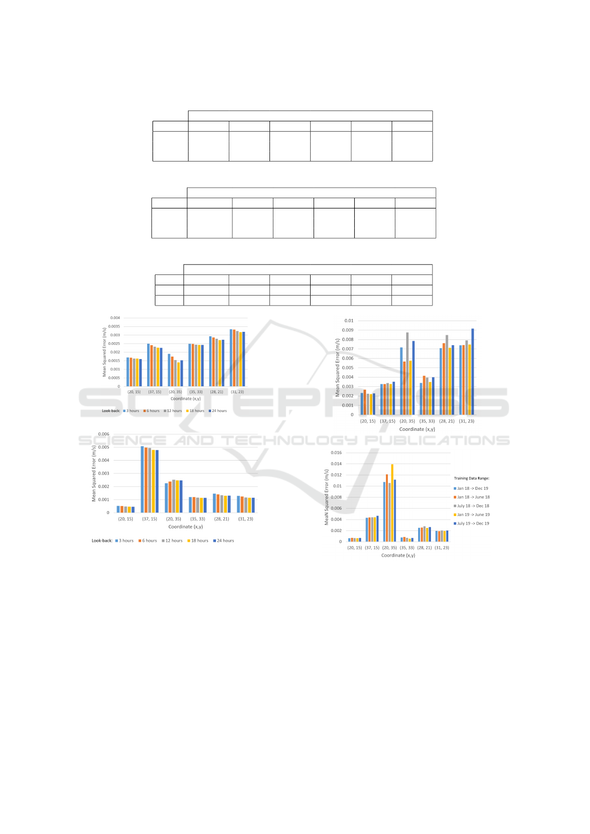
Table 1: Averaged Validation MSE for U Vector Data.
Coordinate
Model (20, 15) (37, 15) (20, 35) 35, 33) (28, 21) (31, 23)
FFNN 0.00176 0.00246 0.00153 0.00252 0.00297 0.00335
LSTM 0.00168 0.00241 0.00174 0.00249 0.00286 0.00332
RF 0.00186 0.00266 0.00148 0.00279 0.00319 0.00360
Table 2: Averaged Validation MSE for V Vector Data.
Coordinate
Model (20, 15) (37, 15) (20, 35) 35, 33) (28, 21) (31, 23)
FFNN 0.000520 0.00508 0.00261 0.00119 0.00144 0.00124
LSTM 0.000509 0.00498 0.00238 0.00120 0.00141 0.00124
RF 0.000562 0.00559 0.00247 0.00129 0.00152 0.00137
Table 3: LSTM Feature Selection Model Averaged Validation MSE.
Coordinate
Data (20, 15) (37, 15) (20, 35) 35, 33) (28, 21) (31, 23)
U 0.00167 0.00240 0.00230 0.00246 0.00283 0.00325
V 0.000506 0.00500 0.00240 0.00118 0.00140 0.00122
(a) U Data MSE Results.
(b) V Data MSE Results.
Figure 1: LSTM Look-Back Comparison Results.
using all data between 01/2018 and 12/2019 was se-
lected as the most appropriate amount of data in order
to train the models since, using all the data rather than
just a 6 month partition, performed slightly better for
most coordinates overall.
4.5 Gap-filling System Overview
The LSTM model configuration having the follow-
ing architecture (6:30:1), obtained improved results
over the other models. This configuration was used
(a) U Data MSE Results.
(b) V Data MSE Results.
Figure 2: LSTM Data Drift Experiment Results.
to train different models on the U and V component
HFR data between 2018 and 2019, for all coordinates
in the raster grid. Figure 3 depicts the gap-filling car-
ried out on data in July 2020. As can be seen from
the map plot, the prediction models manage to learn
trends in the data domain, such as the eddy currents.
When investigating the difference between the actual
and predicted vector values, the differences were al-
ways less than 1m/s which shows that the predictions
were very accurate.
A Novel Approach towards Gap Filling of High-Frequency Radar Time-series Data
235
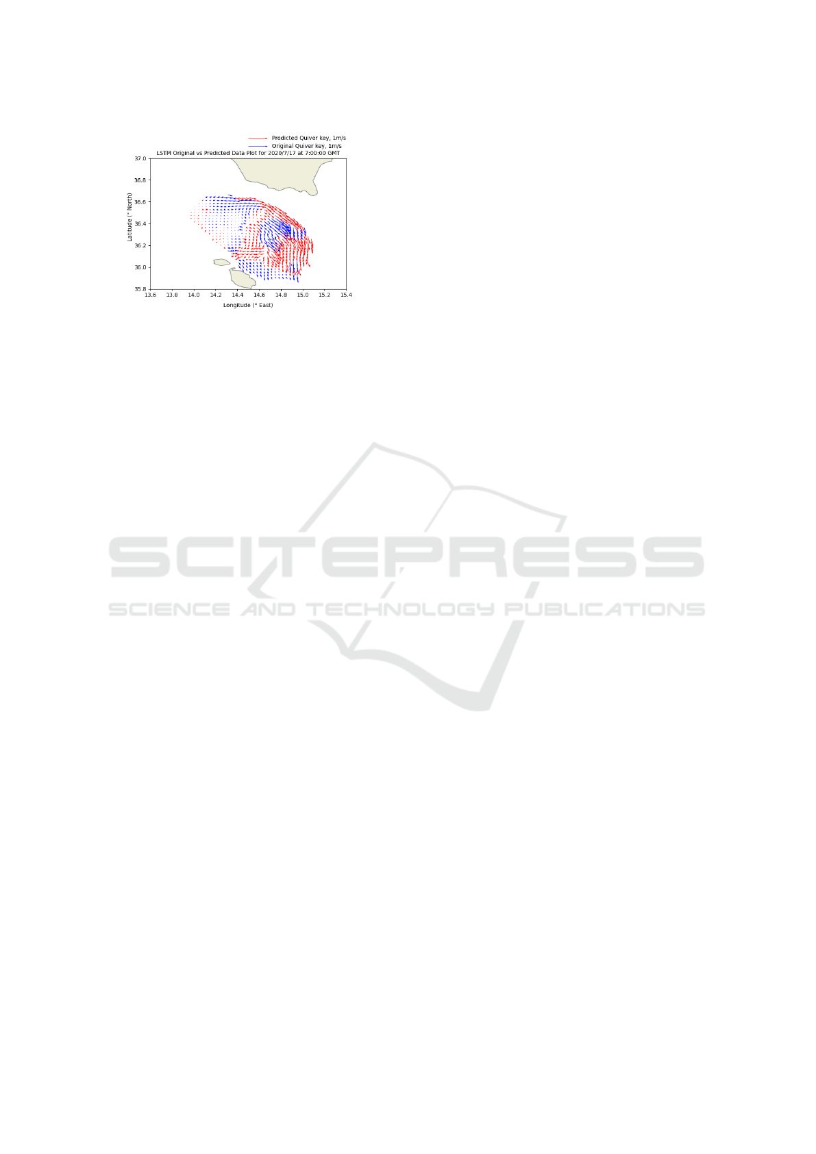
Figure 3: LSTM Gap-Filling Hybrid Model Predictions.
5 CONCLUSION AND FUTURE
WORK
The aim of this research is concerned with achieving
accurate gap-filling of the HFR sea surface current
data through Objectives 1-4. It was discovered that in-
terpolation techniques are not be as accurate as using
machine learning models (Gauci et al., 2016). Fur-
thermore, when comparing the three machine learning
models, the LSTM model was found to be the most
effective.
Furthermore, the addition of external satellite
wind data to the training data did not improve the
results significantly, as discovered by (Vieira et al.,
2020). An investigation was also carried out on the
amount of look-back historical data to use in order to
train the models. Through the experimentation car-
ried out, it was found that using a look-back of six
hours made more sense due to the constraints of the
dataset, as done by (Gauci et al., 2016).
Finally, an investigation was carried out related to
how often the gap-filling models would require re-
training in order to keep them valid for predicting
future data. It was found that there was no drift in
the data when being trained on certain periods. Fur-
thermore, training the models on the full two years
achieved the best results over-all and was able to make
accurate predictions on data in 2020.
5.1 Future Work
Although the wind velocity did not improve the pre-
diction results for gap-filling of the sampled data,
other external features could also be investigated fur-
ther. Tidal elevation and sea surface heights could be
investigated with regards to their effects on the HFR
sea surface current data.
Further investigations on the possibilities of sea-
sonal drift could be investigated further. Models
could be trained on data from different seasons to
test whether any trends in the data are found, and if
models trained per season could achieve more accu-
rate predictions. Finally, this research can be taken
further to achieve short-term forecasting of the HFR
data, which is already in the works.
REFERENCES
Gauci, A., Drago, A., and Abela, J. (2016). Gap filling of
the calypso hf radar sea surface current data through
past measurements and satellite wind observations.
International Journal of Navigation and Observation,
2016.
Karimi, S., Kisi, O., Shiri, J., and Makarynskyy, O. (2013).
Neuro-fuzzy and neural network techniques for fore-
casting sea level in darwin harbor, australia. Comput.
Geosci., 52:50–59.
Kim, Y., Johnson, M. S., Knox, S. H., Black, T. A., Dal-
magro, H. J., Kang, M., Kim, J., and Baldocchi, D.
(2020). Gap-filling approaches for eddy covariance
methane fluxes: A comparison of three machine learn-
ing algorithms and a traditional method with prin-
cipal component analysis. Global Change Biology,
26(3):1499–1518.
Mahjoobi, J. and Adeli Mosabbeb, E. (2009). Prediction of
significant wave height using regressive support vec-
tor machines. Ocean Engineering, 36:339–347.
Pashova, L., Koprinkova-Hristova, P., and Popova, S.
(2013). Gap filling of daily sea levels by artificial
neural networks. TransNav: International Journal on
Marine Navigation and Safety of Sea Transportation,
7:225–232.
Ren, L., Hu, Z., and Hartnett, M. (2018). Short-term
forecasting of coastal surface currents using high fre-
quency radar data and artificial neural networks. Re-
mote Sensing, 10:850.
Sahoo, B., Jha, R., Singh, A., and Kumar, D. (2019).
Long short-term memory (lstm) recurrent neural net-
work for low-flow hydrological time series forecast-
ing. Acta Geophysica, 67.
Song, T., Jiang, J., Li, W., and Xu, D. (2020). A deep
learning method with merged lstm neural networks
for ssha prediction. IEEE Journal of Selected Topics
in Applied Earth Observations and Remote Sensing,
13:2853–2860.
Vieira, F., Cavalcante, G., Campos, E., and Taveira-Pinto,
F. (2020). A methodology for data gap filling in
wave records using artificial neural networks. Applied
Ocean Research, 98:102109.
Wolff, S., O’Donncha, F., and Chen, B. (2020). Statistical
and machine learning ensemble modelling to forecast
sea surface temperature. Journal of Marine Systems,
208:103347.
KDIR 2022 - 14th International Conference on Knowledge Discovery and Information Retrieval
236
