
Using LSTM Networks and Future Gradient Values to Forecast Heart
Rate in Biking
Henry Gilbert, Jules White, Quchen Fu and Douglas C. Schmidt
Vanderbilt University, U.S.A.
Keywords:
Deep LSTM, Deep Neual Network, Heart Rate, Forecasting, Biking.
Abstract:
Heart Rate prediction in cycling potentially allows for more effective and optimized training for a given indi-
vidual. Utilizing a combination of feature engineering and hybrid Long Short-Term Memory (LSTM) models,
this paper provides two research contributions. First, it provides an LSTM model architecture that accurately
forecasts the heart rate of a bike rider up to 10 minutes into the future when given the future gradient values
of the course. Second, it presents a novel model success metric optimized for deriving a model’s accuracy
to predict heart rate while an athlete is zone training. These contributions provide the foundations for other
applications, such as optimized zone training and offline reinforcement models to learn fatigue embeddings.
1 INTRODUCTION
Monitoring intensity during exercise and training is
essential to optimize performance (Sylta et al., 2014).
Insufficient intensity during training yields slower or
negligible performance progression. Excessive in-
tensity, however, yields over-training and the poten-
tial for injury or performance degradation (Collinson
et al., 2001).
There are several metrics for measuring exercise
intensity, including heart rate, V02 max, and power
output (Dooley et al., 2017). Heart rate can be consis-
tently measured across all types of athletics, whereas
power output is exclusive to cycling. Likewise, heart
rate can be used as a reliable indicator of exercise in-
tensity (Jeukendrup and Diemen, 1998). Our intensity
prediction efforts therefore focus on future heart rate.
Yet, predicting heart rate on a given cycling course
is a nuanced and difficult problem. In particular, there
are various external factors that can not be accounted
for, even given the geographical data for a course. For
example, some materials require greater effort to ped-
dle across based on the material’s composition. More-
over, even excluding external course factors, there is
a need to account for cardiac drift, which is a contin-
ual rise or decline of heart rate after exercise due the
body’s internal temperature. (Dawson, 2005). In ad-
dition, there is inconsistency amongst humans, e.g.,
any data derived for training must account for the in-
evitable invariance caused by a person’s inability to
keep perfect pace or other intangible internal factors.
Research Question: Can deep Long Short-Term
Memory (LSTM) models be used to forecast biker
heart rates when given the future gradient val-
ues of the course? The ability for a model to accu-
rately forecast heart rate in the future can potentially
help improve the way athletes approach zone training.
Athletes today typically train reactively, i.e. if during
exercise their heart rate drops too low, they increase
intensity. If their heart rate becomes too high, they
decrease intensity (NEUFELD et al., 2019). This ap-
proach can be a sub-optimal and yield a constantly os-
cillating heart rate and a subsequently greater amount
of time spent outside the correct zone for training.
In contrast, if athletes can accurately predict their
heart rate minutes into the future, they can proactively
adjust their intensity to stay within the desired zone.
For example, if a model forecasts an athlete’s heart
rate will spike out of a given zone due to an upcom-
ing hill in two minutes, the athlete can proactively de-
crease their effort to lower their heart rate to prepare
for the increased effort of the hill. By limiting heart
rate oscillation, the time in the correct zone can in-
crease, thereby optimizing training performance.
Moreover, future heart rate prediction can be ap-
plied to an offline learning model when given enough
contextual data. For example, a model can learn the
embedding of intensity for a given athlete and apply
that learning to optimally indicate when the athlete
should speed up or slow down to ensure their heart
rate remains in a given zone. This is a novel ap-
proach that fundamentally contrasts with a coach re-
Gilbert, H., White, J., Fu, Q. and Schmidt, D.
Using LSTM Networks and Future Gradient Values to Forecast Heart Rate in Biking.
DOI: 10.5220/0011541800003321
In Proceedings of the 10th International Conference on Sport Sciences Research and Technology Support (icSPORTS 2022), pages 53-60
ISBN: 978-989-758-610-1; ISSN: 2184-3201
Copyright
c
2022 by SCITEPRESS – Science and Technology Publications, Lda. All rights reserved
53

Figure 1: Model Results for 120’s Prediction on Validation
Run 0.
actively instructing an athlete. Therefore, an indepen-
dent model can optimally and proactively dictate an
athlete’s intensity. This information could be commu-
nicated to an athlete in the form of a [1,10] intensity
scale, with 1 being minimum effort and 10 being max-
imum effort, thereby potentially maximizing training
for an athlete’s specific intensity embeddings.
Key Contribution: A promising deep LSTM
Model for predicting heart rate Up to 600 seconds
in the future. This paper presents an architecture for
an LSTM model (Hochreiter and Schmidhuber, 1997)
that can predict heart rate up to 600 seconds (i.e., 10
minutes) in the future. This LSTM model achieves
this predictability via a mix of past historical heart
rate and velocity data with the future gradient values
of the course n minutes into the future.
The remainder of this paper is organized as fol-
lows: Section 2 summarizes related work and ex-
plores its relationship with the research described in
this paper; Section 3 illustrates the models underlying
architecture and the reasoning behind it; Section 4 ex-
plains the model’s performance in relation to the ex-
perimental data and analyzes the experiment results;
and Section 5 presents concluding remarks.
2 RELATED WORK
Prior work exploring heart rate prediction using ma-
chine learning can be categorized as focusing on (1)
predicting heart rate given noisy data and (2) forecast-
ing heart rate in the context of sports. This section
summarizes this related work and explores its rela-
tionship with the research described in this paper.
An important problem in the analysis of heart rate
is the quality of the data being collected. Unfor-
tunately, due to external factors (such as sweat and
excessive motion during exercise) common sensors
(such as PPG and ECG) fail to produce accurate read-
ings. Recent work has applied machine learning to
forecast heart rate more accurately, regardless of the
noise within the input data.
Figure 2: Model Results for 120’s Prediction on Validation
Run 1.
For example, (Yun et al., 2018) focused on fore-
casting heart rate variability via a Hidden Markov
model. Likewise, (Fedorin et al., 2021) compared
sequence-to-sequence models and deep LSTM mod-
els with integrated CNN layers for more accurate
heart rate forecasting and concluded that LSTM
model performed marginally better than the sequence-
to-sequence model. In contrast, our work focuses on
a related—but different—application, ı.e., ingesting
and forecasting using noisy data to predict heart rate
in the context of biking, rather than subjects at rest.
A recent paper (Staffini et al., 2022) uses the past
n minutes of heart rate data to predict heart rate at
n + 1. Using only an auto-regressive model, this pa-
per achieved an mean absolute error (MAE) of 3 bmp.
However, once again, that paper’s data set consisted
entirely of subjects at rest. Thus, their model allowed
less variance in the external environment when com-
pared to heart rate forecasting in an exercise setting,
such as our focus on biking in this paper.
Yet another recent paper (Ni et al., 2019) com-
bined LSTM with sequence-to-sequence and encod-
ing layers to create a workout forecasting model,
a short-term heart rate forecaster, a linear projec-
tion embedding module, and a workout recommender
system. Given contextual information about the
user’s historical performance and sport type, they
constructed a model to forecast the user’s heart rate
for a given workout route at minute intervals. The
short-term forecasting model used a custom encoder-
decoder with temporal attention to forecast heart rate
10’s ahead with a resulting root means square error
(RMSE) of 7.025 heart beats. In contrast, our work
focuses on heart rate in the context of biking and
specifically applying future gradient values of a given
course for predictions up to 600 seconds ahead.
Finally, one of our earlier papers (Qiu et al., 2021)
is based on the same data set as this paper and also
forecasts heart rate at a one second interval using
several models, including Random Forest, a Feed-
Forward Neural Network (FFNN), a Recurrent Neu-
ral Network (RNN), and LSTM. That paper found
icSPORTS 2022 - 10th International Conference on Sport Sciences Research and Technology Support
54

Figure 3: Model Results for 120’s Prediction on Validation
Run 2.
Figure 4: Model Results for 120’s Prediction on Validation
Run 3.
the LSTM model exhibited the top forecasting per-
formance out of the aforementioned models. While
that paper shared a similar research question and the
same data set as our current paper, the papers differ
in two ways: (1) our current paper introduces a novel
forecasting performance metric to relate predictions
to their heart rate zone and (2) it also applies future
gradient values to increase the LSTM model’s predic-
tive power and ability to generalize.
3 MODEL ARCHITECTURE
This section describes the LSTM architecture that we
analyzed in our experiments to predict future heart
rate values given the future gradient values. Figure 5
shows the overall architecture for the LSTM model
that produced the best results, which consisted of 5
layers of 1000 neurons each. We experimented with
a variety of layers and neurons. Specifically, we ex-
perimented with models ranging from 2 layers of 50
neurons to models with 10 layers of 5,000 neurons.
Two additional dense layers were appended to the end
of the model to learn the output embedding from the
LSTM layers and apply it to forecast the heart rate.
Our experiments indicated that smaller models
were unable to capture the complexity of the rela-
tionships present in the data. Such models would
often end up converging to the average heart rate of
the training set, rather than a mapped relationship be-
tween gradient and heart rate. Conversely, models
larger than 5 layers of 1,000 neurons often had di-
minishing returns and struggled with over fitting the
training data. Thus, they were not worth the exponen-
tial increase in compute time.
For heart rate prediction, our LSTM model used
three input vectors: past heart rate, past cadence, and
future gradient. All data was normalized between
[0,1]. Each of these vectors were bucketed and aver-
aged by chunks of five to reduce the input space and
limit the noise found in such granular data.
Chunk size was determined via grid search exper-
imentation, where we experimented with values in the
range of [1,2,5,10,50,100]. A chunk size of five con-
clusively performed the best. In particular, this chunk
size optimally balanced between retained information
density and noise reduction through smoothing.
These three vectors were then interwoven into
each other such that given vector heart rate =
[h
0
,h
1
,h
2
], vector cadence = [c
0
,c
1
,c
2
] and vector
gradient = [g
3
,g
4
,g
5
]. The resulting vector was then
[h
0
,c
0
,g
3
,h
1
,c
1
,g
4
h
2
,c
2
,g
5
]. The heart rate and ca-
dence are historical values, while the gradient is the
future gradient of the route.
This interwoven list was subsequently segmented
into chunks of six, such that the model took a depth of
six steps for every feature vector x ∈ X. Given histor-
ical data h
0
, ... ,h
n
, c
0
, ... ,c
n
and g
0
, ... ,g
n
, the model
predicted the heart rate at time step 2n. Specifically,
for a prediction 120 seconds into the future, the in-
put was reformatted into chunks of the previous 120’s
of heart rate and cadence, along with the future 120’s
of the gradient. Given 120’s chunk of historical data,
[t
0
,t
120
] was used to make a singular prediction, 120’s
into the future at time step t
240
. Thus, given heart rate
= [h
0
,..., h
120
], cadence = [c
0
,..., c
120
] and gradient =
[g
120
,..., g
240
], the model predicted the heart rate of
the athlete at time step t
240
.
Our approach interwove past heart rate, past ca-
dence, and future gradient together to enable the seg-
mentation of time steps when the data was fed to
the model. If heart rate, cadence, and gradient were
merely appended to the end of each other that data
could not be segmented into time steps because the
first step would consist entirely of heart rate data, the
last step would consistent entirely of gradient values,
and the rest would be a mix of all three. To achieve
consistent and homogeneous time steps the three data
vectors must be interleaved.
Our LSTM model’s input layer took batch sizes of
one, where each time-step had a feature vector of size
of size 10. There were model − look − f orward −
amount/10 time-steps for each input into the model.
Using LSTM Networks and Future Gradient Values to Forecast Heart Rate in Biking
55

Figure 5: Model Architecture.
This part of the algorithm yielded a many-to-one
LSTM input architecture.
This input was then fed into four subsequent and
identical LSTM layers, each with 1,000 neurons. Ev-
ery one of these hidden LSTM layers had a 0.2 in-
tegrated drop layer. This portion of the algorithm
yielded a trainable 800 neurons, per layer, per pass.
The output of the deep LSTM model was then fed
into a densely connected layer of 800 neurons. The
subsequent output from this layer was next fed into
two further densely connected hidden layers with 300
neurons each. Finally, the output was condensed into
a final single neuron with a linear activation applied
to forecast the heart rate.
Our LSTM model utilized a mean absolute error
loss function. Specifically, the absolute value of the
forecasting errors are summed together and used to
adjust the networks weights, as shown in Equation 1.
D
∑
i=1
|x
i
− y
i
|
Equation 1: Mean absolute error function.
As described previously, the model also applied a
custom metric to determine model forecasting success
in relation to heart rate zones. Specifically, to calcu-
late the error between actual heart rate and predicted
heart rate, this metric created a relative error to the
size of the heart zone, which distinguished between
upper and lower bounds of a given zone and related
the distinction to the actual size of that zone.
For example, given a heart rate zone between 200
and 180 beats per minute the size of this heart rate
zone is 20 beats. Therefore, if the actual heart rate is
185 and the predicted heart rate is 190 the actual error
is 5 beats. Given this zone size 20, the adjusted error
is 5/20 or 0.25.
In contrast, for a heart zone between 200–190 with
a zone size of 10 the actual error is also 5 beats if the
actual heart rate is 195 and the predicted heart rate is
200. In this case, however, the adjusted error becomes
5/10 or 0.5. Since the zone is smaller, the relative dif-
ference between actual and predicted heart rate carries
a greater impact.
The difference in importance using the concrete
error cannot be captured in this scenario. However,
the relative adjusted error does capture this discrep-
ancy in importance. This distinction is shown by the
concrete error being 5 beats for both examples, but a
higher adjusted error of 0.5, rather than 0.25. This dif-
ference compensates for the narrower margins of the
smaller heart rate zone.
4 EXPERIMENT METHODS AND
RESULTS
This section gives an overview of our experiment data
and training method, analyzes the results from our ex-
periments, and explains threats to validity.
4.1 Overview of the Experiment
The data set used to train LSTM model comprised the
grade of the course, speed, heart rate, elevation, dis-
tance and cadence, all measured at one second inter-
vals. There were 110 overall rides, resulting in a data
set of 270,000 examples. We used both a validation
set of 30k examples and the same validation set de-
scribed in (Qiu et al., 2021) to directly contrast model
performance more accurately.
Our LSTM model was trained on a machine with
48GB of VRAM and 256GB RAM. This model uti-
lized early stopping with a patience of five and a min-
imum value loss variance of one. The model ran for
an average of eight epochs at a training time of four
minutes each, resulting in an average training time of
32 minutes.
icSPORTS 2022 - 10th International Conference on Sport Sciences Research and Technology Support
56

4.2 Analysis of Data
Understanding the nature and quality of the data is
essential before a full analysis of the results can be
given. Firstly, to give context to the model’s accuracy,
one must calculate the variance within the data.
Specifically, the variance of the heart rate data
is: 604.489, and the variance of the cadence data is:
1200.718. Both variance were derived using Formula
2. Naturally, variance relates to the scale of the data
it was derived from. However, even accounting for a
max heart rate of 219 and a max cadence of 225, both
data sets variance is relatively high. Cadence having
a high variance can be attributed to the the athlete’s
inability to hold a constant pace, along with the nat-
ural increase and decrease of effort in relation to the
course’s changing gradient. The high variance in the
heart rate can be attributed to an athlete’s imperfect
pace, along with the corresponding athlete’s ability
for physiological heart rate control. These factors are
echoed in the covariance between cadence and heart
rate, 221.204, and the correlation between cadence
and heart rate, 0.251. With correlation being calcu-
lated with Equation 3.
Thus, a large variance in both heart rate and ca-
dence helps form an upper ceiling for expected model
forecasting accuracy. The model will not only have
to model future heart rate for a given course, but also
account for the non-deterministic human divergence
from constant pace.
σ
2
=
n
∑
i=1
(x
i
− µ)
2
n
Equation 2: Variance equation.
r =
∑
n
i=1
(x
i
− x)(y
i
− y)
p
∑
n
i=1
(x
i
− x)
2
(y
i
− y)
2
Equation 3: Pearson’s R equation.
4.3 Analysis of Results
A concrete example of the model’s performance on a
single ride is shown in Figure 6. Exact model perfor-
mance for each ride in the validation set is shown in
Table 1.
The corresponding run graph results are shown in
Figures 1, 2, 3, 4, 7, 8, 9, 10, 11 12. Given the valida-
tion set of 30k examples, the model achieves a mean
squared loss of 25.63, though there are outliers around
step 5,000 in the validation set. Regardless of the in-
herent noise in the data, the model continues to fit
Figure 6: Model Results for 120’s prediction across valida-
tion set of 30,000 data points.
Table 1: Model Performance on Validation Rides.
Validation Ride MAE RZE
Run 0 13.82 0.47
Run 1 21.61 1.07
Run 2 23.23 1.04
Run 3 22.99 0.86
Run 4 32.34 1.52
Run 5 19.17 0.83
Run 6 14.84 0.58
Run 7 23.29 0.71
Run 8 22.67 1.02
Run 9 32.54 0.98
the general trend and not diverge to only predicting
the most recent heart rate. These results showcase the
model’s ability to learn the relationship between cur-
rent heart rate and future gradient values.
This same model can then be retrained to predict
10 minutes into the future. Even predicting so far into
the future, the model still generalizes to the correct
trend, as shown in Figure 13.
The 10 minute model’s predictions fail to contin-
ually match the trend of the users heart rate across
the entirety of the 2,000 time steps. However, this
result shows the model’s ability to learn the strong re-
lationship between past heart rate and cadence values
to future gradient values. Moreover, the divergence in
accuracy between time steps 750 and 1,250 can be ex-
plained by an analysis of the user’s cadence during the
same time period. As shown in Figure 14, the cadence
Figure 7: Model Results for 120’s Prediction on Validation
Run 4.
Using LSTM Networks and Future Gradient Values to Forecast Heart Rate in Biking
57
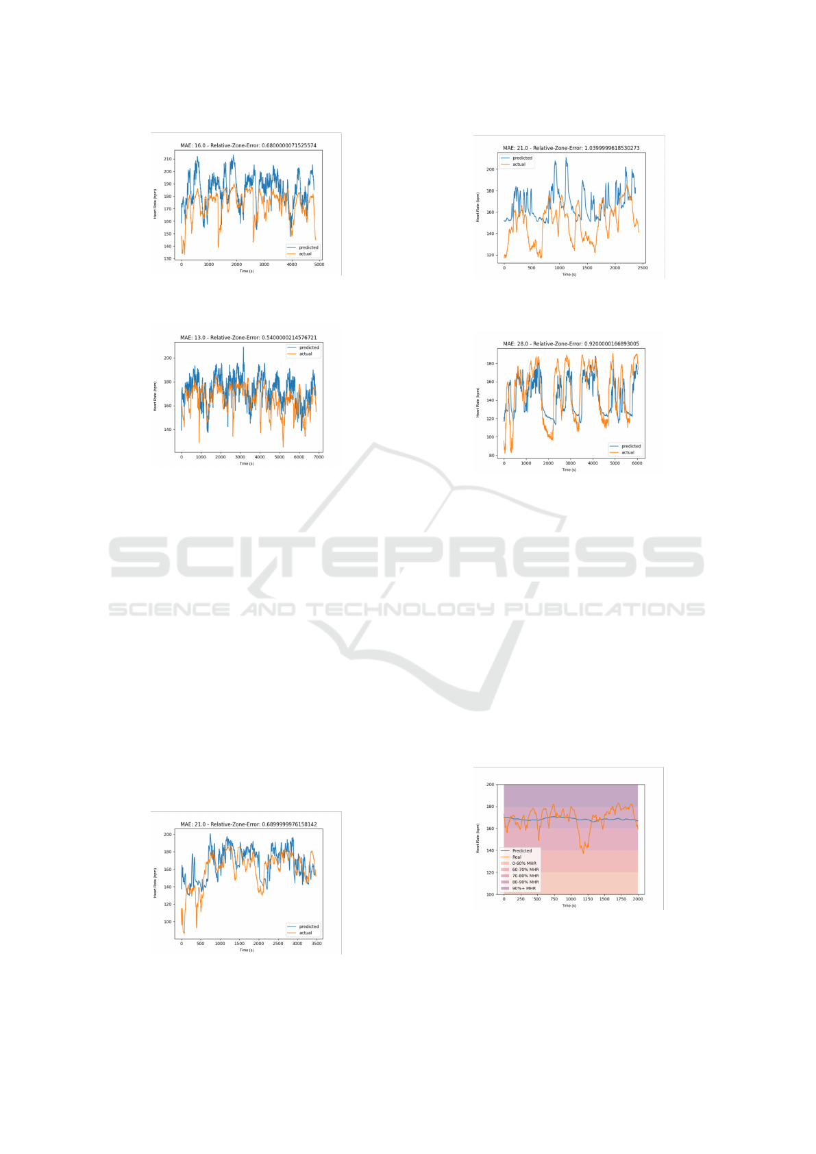
Figure 8: Model Results for 120’s Prediction on Validation
Run 5.
Figure 9: Model Results for 120’s Prediction on Validation
Run 6.
drops to 0, suggesting the athlete stopped during the
user’s ride.
Naturally, the model can not account for an un-
expected departure of the course and the subsequent
cardiac drift that ensues. However, the model was
quickly able to refit the trend, as shown in Figure 13.
Moreover, Figure 15 depicts forecasting heart rate at
120’s intervals in relation to the associated heart rate
zones for the given athlete.
This model can therefore make valuable and ac-
tionable predictions if it is able to fit the trend of heart
rate zones, which is not necessarily a direct trend
with the heart rate. It is also essential to consider the
model’s confidence bounds, as shown in Figure 16.
Allowing for a certain margin of uncertainty in the
model’s predictions yields a better generalization to-
wards predicting zone relations. Specifically, this re-
lationship can be quantified to zone trends by taking
Figure 10: Model Results for 120’s Prediction on Validation
Run 7.
Figure 11: Model Results for 120’s Prediction on Validation
Run 8.
Figure 12: Model Results for 120’s Prediction on Validation
Run 9.
the absolute difference in a model’s prediction and the
ground truth and then scaling the difference to the size
of an individuals heart rate zone. For reference, the
model seen in 15 has an average relative zone error of
0.414, so it is accurate to within 60 percent of a given
heart zone for any x ∈ X. Figure 13 and Figure 17.
An example of the importance for generalized
zone forecasting instead of granularity heart rate is
shown in 13 It initially appeared the 10 minute model
was unable to fit the validation set as well as as the
two minute model. However, the 10 minute model
sacrificed granular tracking for a more robust relation-
ship with the given zone for a heart rate. This trade off
allowed the model to achieve a lower relative zone er-
ror score of 0.37.
Figure 13: Model Results for 600’s Predictions.
icSPORTS 2022 - 10th International Conference on Sport Sciences Research and Technology Support
58
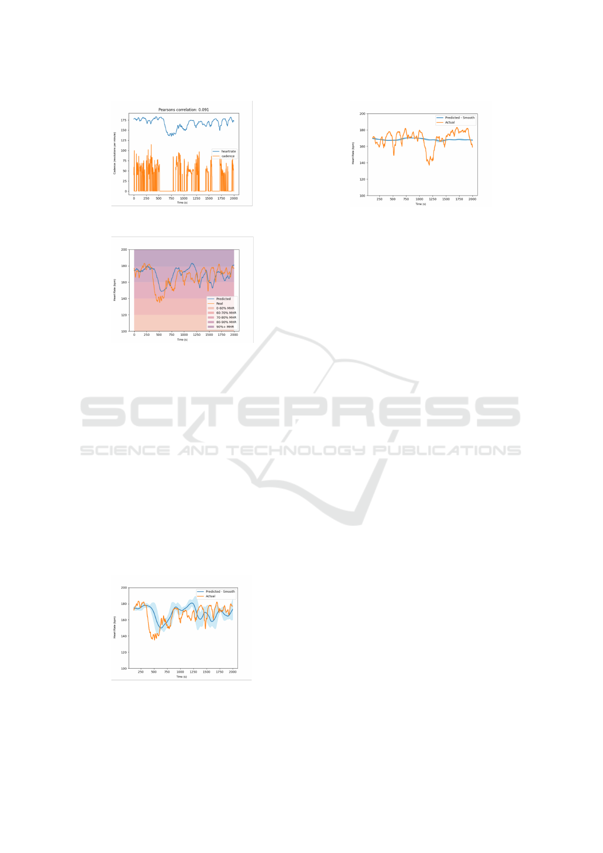
Figure 14: Cadence in Relation to Heart Rate.
Figure 15: 120’s Prediction for Single Ride in Reference to
Training Zones.
4.4 Threats to Validity
The results reported above show that our LSTM
model’s utility for optimized heart rate zone training
is promising and potentially actionable. However, the
current data set consists of only one athlete cycling
on a multitude of different routes and has not yet been
tested on other individuals cycling on more diverse
routes and in other sport types, such as running. Intu-
itively, this model should generalize to a greater pop-
ulation of subjects and contexts as the model’s inputs
are agnostic of the route, person or sport type. It also
remains an open research question if the model can
generalize across an entire population of athletes or if
each individual athlete will need a model fine-tuned
to their internal exertion embeddings.
Figure 16: 120’s Prediction in reference to it’s confidence
intervals.
Figure 17: 600’s Prediction in reference to it’s confidence
intervals.
5 CONCLUDING REMARKS
Few papers have been published that provide deep
learning model architectures for forecasting heart rate
more than 60 seconds into the future. As discussed
in Section 2, even fewer proposed models attempt to
forecast heart rate in an athletic context.
This paper showed that a hybrid LSTM model in
conjunction with supplying future gradient values for
a given course allows prediction of actionable heart
rate forecasts up to 10 minutes into the future. Specif-
ically, by feeding a deep LSTM model into a densely
connected deep neural network, we are able to accu-
rately forecast the heart rate of an athlete biking in re-
lation to the gradient values of a given course. These
results suggest other potential applications for opti-
mized zone training and offline learning for athlete
intensity management through exertion embeddings.
Our research reported in this paper yield the fol-
lowing lessons regarding forecasting heart rate in an
athletic context:
1. LSTM Architecture for Heart Rate Forecast-
ing. As shown in this paper, the LSTM model
architecture is an effective choice for forecasting
future heart values.
2. Increased Forecasting Ability with Future
Gradient Values. Our LSTM model effectively
predicted the heart rate of an athlete up to 10 min-
utes into the future when using the future gradient
values of the course. This result demonstrated the
strong predictive relationship between the gradi-
ent of a course and heart rate.
3. Adjusted Model Success Metrics. We learned
that adjusting the model prediction error in rela-
tion to the size of a heart rate zone is a more de-
scriptive metric to define model success.
Our future work will continue evolving this re-
search by performing larger experiments with a more
diverse subject group to gain a greater breadth of
Using LSTM Networks and Future Gradient Values to Forecast Heart Rate in Biking
59

data. Specifically, we will increase our sample size by
studying 20 different athletes of an even distribution
of gender, as well as have each athlete cycle 10 differ-
ent routes and run the same 10 routes. We will then
use this data to retrain a larger version of the current
LSTM model and test whether this model can effec-
tively learn the relationship between future gradient
and current heart rate, irrespective of an athlete’s gen-
der, fitness level, or sport.
All of the models and data that we presented in
this paper can be downloaded in open-source form
at the following GitHub repository URL: github
.com/henrygilbert22/RL-Human-Performance.
Please consult the repo’s ReadMe file for in-depth
instructions on replicating this paper’s results and a
more extensive description of the data used in the
experiments.
REFERENCES
Collinson, P. O., Boa, F. G., and Gaze, D. C. (2001). Mea-
surement of cardiac troponins. volume 38, pages 423
– 449.
Dawson, E. A. (2005). Cardiac drift during prolonged ex-
ercise with echocardiographic evidence of reduced di-
astolic function of the heart. volume 94, page 3.
Dooley, E. E., Golaszewski, N. M., and Bartholomew, J. B.
(2017). Estimating accuracy at exercise intensities:
A comparative study of self-monitoring heart rate and
physical activity wearable devices. JMIR Mhealth
Uhealth, 5(3):e34.
Fedorin, I., Slyusarenko, K., Pohribnyi, V., Yoon, J., Park,
G., and Kim, H. (2021). Heart rate trend forecasting
during high-intensity interval training using consumer
wearable devices. In Proceedings of the 27th Annual
International Conference on Mobile Computing and
Networking, MobiCom ’21, page 855–857, New York,
NY, USA. Association for Computing Machinery.
Hochreiter, S. and Schmidhuber, J. (1997). Long short-term
memory. Neural Comput., 9(8):1735–1780.
Jeukendrup, A. and Diemen, A. V. (1998). Heart rate moni-
toring during training and competition in cyclists. vol-
ume 16, pages 91–99.
NEUFELD, E., WADOWSKI, J., BOLAND, D., Dolezal,
B., and Cooper, C. (2019). Heart rate acquisition and
threshold-based training increases oxygen uptake at
metabolic threshold in triathletes: A pilot study. In-
ternational Journal of Exercise Science, 12:144–154.
Ni, J., Muhlstein, L., and McAuley, J. (2019). Modeling
heart rate and activity data for personalized fitness rec-
ommendation. In The World Wide Web Conference,
WWW ’19, page 1343–1353, New York, NY, USA.
Association for Computing Machinery.
Qiu, X., White, J., and Schmidt, D. C. (2021). Analyz-
ing machine learning models that provide personal-
ized heart rate forecasting for elite cyclists.
Staffini, A., Svensson, T., Chung, U.-i., and Svensson, A. K.
(2022). Heart rate modeling and prediction using au-
toregressive models and deep learning. volume 22.
Sylta, y., Tønnessen, E., and Seiler, S. (2014). From heart-
rate data to training quantification: A comparison of 3
methods of training-intensity analysis. International
journal of sports physiology and performance, 9:100–
7.
Yun, S., Son, C.-S., Lee, S.-H., and Kang, W.-S. (2018).
Forecasting of heart rate variability using wrist-worn
heart rate monitor based on hidden markov model. In
2018 International Conference on Electronics, Infor-
mation, and Communication (ICEIC), pages 1–2.
icSPORTS 2022 - 10th International Conference on Sport Sciences Research and Technology Support
60
