
Automatic Feature Extraction for Bearings’ Degradation Assessment
using Minimally Pre-processed Time series and Multi-modal Feature
Learning
Antonio L. Alfeo
1,2
, Mario G. C. A. Cimino
1,2
and Guido Gagliardi
1,3,4,∗
1
Department of Information Engineering, University of Pisa, Pisa, Italy
2
Bioengineering and Robotics Research Center E. Piaggio, University of Pisa, Pisa, Italy
3
Department of Information Engineering (DINFO), University of Florence, Florence, Italy
4
Department of Electrical Engineering, KU Leuven, Leuven, Belgium
Keywords:
Feature Learning, Data Fusion, Deep Learning, Multimodal Autoencoder, Contrastive Learning, Predictive
Maintenance, Smart Manufacturing.
Abstract:
Maintenance activities can be better planned by employing machine learning technologies to monitor an asset’s
health conditions. However, the variety of observable measures (e.g. temperature, vibration) and behaviours
characterizing the health degradation process results in time-consuming manual feature extraction to ensure
accurate degradation stage recognitions. Indeed, approaches able to provide automatic feature extraction from
multiple and heterogeneous sources are more and more required in the field of predictive maintenance. This is-
sue can be addressed in a data-driven fashion by using feature learning technology, enabling the transformation
of minimally processed time series into informative features. Given its capability of discovering meaningful
patterns in data while enabling data fusion, many feature learning approaches are based on deep learning
technology (e.g. autoencoders). In this work, an architecture based on autoencoders is used to automatically
extract degradation-representative features from minimally preprocessed time series of vibration and temper-
ature data. Different autoencoder architectures are implemented to compare different data fusion strategies.
The proposed approach is tested considering both the recognition performances and the quality of the learned
features with a publicly available real-world dataset about bearings’ progressive degradation. The proposed
approach is also compared against manual feature extraction and the state-of-the-art technology in feature
learning.
1 INTRODUCTION
The paradigm known as Industry 4.0 recommends
the integration of machine learning in industrial pro-
cesses to improve them (Alfeo et al., 2021) and avoid
production inefficiencies (Alfeo et al., 2020). Re-
garding the maintenance procedures, such technolo-
gies are enabling the so-called Predictive Mainte-
nance (PdM) (Jimenez et al., 2020). PdM aims at
driving the maintenance operations to execute them
just before the breaking point rather than after a fail-
ure or according to some regular schedule. This al-
lows avoiding the costs due to a failure while still ex-
ploiting the whole remaining useful life (RUL) of an
asset’s component (Wan et al., 2017).
∗
Corresponding author
RUL predictions are often unreliable since they
are greatly affected by the usage of the assets while
in an unhealthy stage (Lei et al., 2018). For this rea-
son, many real-world applications provide degrada-
tion stage estimations rather than RUL predictions.
The number of stages characterizing the degra-
dation process results from a trade-off between the
interpretability of the prediction and the complex-
ity of the degradation process. The more the asset’s
degradation process is consistent and progressive, the
more it can be effectively modeled with a few easy-
to-interpret stages. Most of the research works (Lei
et al., 2018) divide the degradation process into three
(Vinh et al., 2009), others into four (Scanlon et al.,
2012), or even five stages (Kimotho et al., 2013).
However, due to the many possible measures to
monitor an asset’s health condition, and the diversity
94
Alfeo, A., Cimino, M. and Gagliardi, G.
Automatic Feature Extraction for Bearings’ Degradation Assessment using Minimally Pre-processed Time series and Multi-modal Feature Learning.
DOI: 10.5220/0011548000003329
In Proceedings of the 3rd International Conference on Innovative Intelligent Industrial Production and Logistics (IN4PL 2022), pages 94-103
ISBN: 978-989-758-612-5; ISSN: 2184-9285
Copyright
c
2022 by SCITEPRESS – Science and Technology Publications, Lda. All rights reserved

of the degradation processes across industries and ma-
chines, it is difficult to provide a high-quality feature
extraction process that is also generalizable among
different PdM applications (Ran et al., 2019). More-
over, both too many redundant features and a few less
informative ones (i.e. that do not ease the distinction
between the behaviors under analysis), may degrade
the performance of algorithms using them (Lorena
et al., 2019). This results in a time-consuming collab-
oration between data scientists and maintenance ana-
lysts to manually transform raw signals into informa-
tive features for application-specific PdM approaches.
In this context, a less manual feature extraction pro-
cess is more and more needed (Yan and Yu, 2015),
and this can be achieved by employing feature learn-
ing approaches (Bengio et al., 2013). Contrary to
manual knowledge-driven feature extraction (Parola
et al., 2022), feature learning is an integrated learn-
ing process in which algorithms learn to automatically
transform minimally processed data into informative
features able to simplify a classification task (Vincent
et al., 2010). Feature learning does not necessarily
require prior domain knowledge, e.g. which features
to select and which to eliminate, and it can be done
by explicitly maximizing the relationship between the
learned features and the target classes.
In this context, the capability of automatically ex-
tracting informative features from multiple and het-
erogeneous sources is more and more required in the
field of predictive maintenance (Lei et al., 2018). The
convenience of multi-modal ML approaches for PdM
is indeed emphasized in different recent surveys such
as (Merkt, 2019). This type of data is coming from
multiple sensors, which normally would require a
specific preprocessing and feature extraction for each
one of them. The use of a feature learning approach
can therefore be a valid solution to handle this kind of
data effectively.
Many recent multi-modal feature learning ap-
proaches are based on deep learning technology
(Zhong et al., 2019), and especially on deep autoen-
coders (AE) (Ran et al., 2019). Indeed, by being char-
acterized by hierarchically stacked nonlinear mod-
ules, deep learning enables the simultaneous process-
ing of data from different sources or modalities while
providing a higher-level representation of the inputs
that can be used as features in a classification prob-
lem. This study aims to compare the complexity
and accuracy of different AE architectures for mul-
timodal feature learning and to exploit those with a
well-known PdM benchmark dataset. For instance,
concatenating the features obtained by training one
AE for each modality may result in a longer training
time whereas concatenating the modalities results in
a more complex AE architecture. The contribution of
this work can be summarized as:
• an architecture to learn degradation-representative
features by providing a deep autoencoder-based
with minimally preprocessed time series of vibra-
tion and temperature data;
• a comparison of different variations of the autoen-
coder architecture to implement different data fu-
sion strategies;
• an assessment of the quality of the learned fea-
tures and recognition performances with respect
to the classic feature extraction and the state of
the art technology in feature learning;
The proposed approach has been tested on 3 real-
world cases study characterizing the degradation of
industrial bearings via their temperature and vibra-
tion. The paper is structured as follows. In section
2, the literature review is presented. Section 3 details
the proposed approach. The case study and the ex-
perimental setup are presented in sections 4. Finally,
section 5 and 6 discuss the obtained results and the
conclusions, respectively.
2 RELATED WORKS
In this section, a survey of the state of the art is
presented. It addresses deep learning-based feature
learning with a focus on approaches based on multi-
modal feature learning. Deep learning approaches
have proven to be effective at providing a non-linear
combination of the input data to distill higher-level in-
formation, i.e. automatically learning features (Tang
et al., 2019).
A deep learning architecture is built by stacking
layers of artificial neurons (Gao et al., 2020). The
inputs provided to the architecture are processed by
each layer, thus each layer produces the features for
the next one. This processing is guided by a loss func-
tion that minimizes a target error. Thus, is intrinsi-
cally a feature learning approach, although depend-
ing on the loss used, features may be more or less
useful for feature extraction. For instance, the most
used deep learning architecture for feature-learning is
the so-called autoencoder (AE), which has proven its
convenience in learning latent feature representation
in many application domains (Deng, 2014).
AE is made of two main components: the en-
coder produces a compact representation of the in-
puts, whereas the decoder reconstructs the input data
from such a compact representation. The AE net-
work is then trained through a loss function that max-
imizes the similarity between its input and output, re-
Automatic Feature Extraction for Bearings’ Degradation Assessment using Minimally Pre-processed Time series and Multi-modal Feature
Learning
95
sulting in a completely unsupervised approach. Once
trained the compact representation provided by the
encoder can be used as a feature for classification
tasks. Specifically designed to be fed by different in-
puts, the so-called multimodal autoencoder can fuse
multi-sensory data while performing feature learning
(Yan et al., 2020).
When based on autoencoders, it is possible to pro-
vide a feature learning approach with a data fusion
mechanism in 3 different ways (Gao et al., 2020):
• Data-level Fusion: these approaches learn a
multi-modal feature representation by processing
the concatenation of the original input data for
each modality (Gecgel et al., 2022).
• Architecture-level Fusion: these approaches learn
a multi-modal feature representation by process-
ing each modality independently, up to the last
layers of the neural network architecture that are
shared among the different modalities (Shin et al.,
2021).
• Representation-level Fusion: these approaches
learn a multi-modal feature representation by pro-
cessing independently each modality and concate-
nating the representation learned from each one of
them (Alfeo et al., 2022).
As an example, in (Ngiam et al., 2011) many
AE deep learning approaches for handling multi-
modal audio-video features are proposed and dis-
cussed. In particular, the so-called shared modality
AEs which take concatenated multi-modal features as
input and reconstruct them (data-level Fusion), and
multi-Modal AEs which are multi-input-multi-output
networks (Architecture-level Fusion), in which one
modality is provided at each input level and processed
by the network together with the others and then re-
constructed separately at each output level.
Alternatively, to feature learning approaches
based on AE, a neural network can directly learn
a new set of features by employing specifically de-
signed loss functions. An example of this is the
multi-similarity loss provided by Tensorflow Simi-
larity (Elie Bursztein, 2021) which represents the
state-of-the-art learning features for similarity rank-
ing problems. This approach is based on learning
a representation in the latent space that clusters the
samples belonging to the same class while maximiz-
ing the distance between samples belonging to dif-
ferent classes. This results in a fully supervised fea-
ture learning approach. The main difference between
these two approaches is that AE tries to learn a new set
of features that is informatively identical to the origi-
nal one so that it can be reconstructed correctly, simi-
larity encoder instead learns a new set of features that
maximize their separability in correspondence with
the target classes.
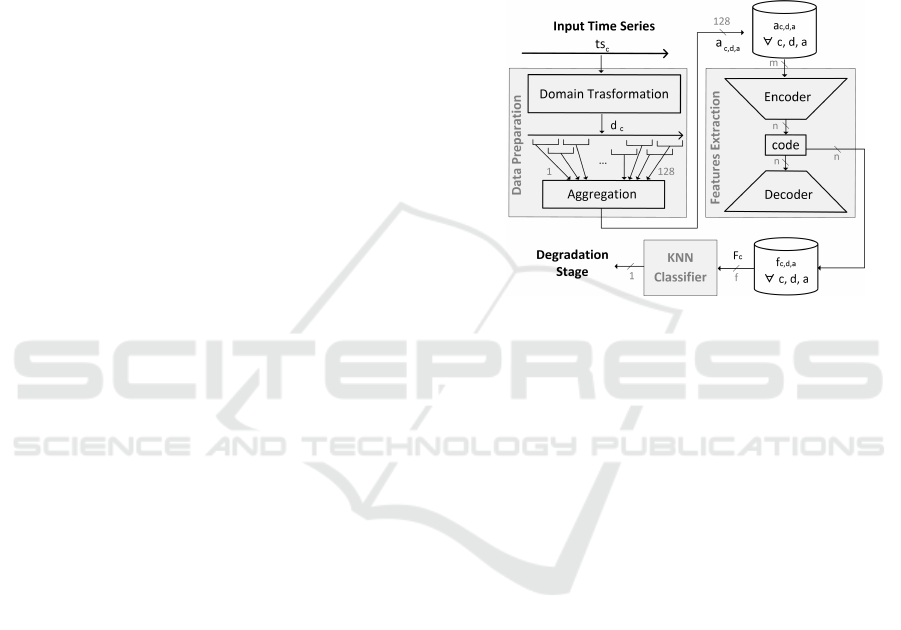
3 DESIGN
In this section, the design of the proposed approach is
detailed. It consists of three functional modules, i.e.
data preparation, feature extraction, and degradation
stage recognition.
Figure 1: Architecture of the proposed approach.
The data preparation module provides the mini-
mal preprocessing needed to use them as inputs for
the feature extraction module. The vibration and
temperature time series are segmented using semi-
overlapping time windows with a duration of 30 sec-
onds. Each segment ts
c
is associated with a degra-
dation stage (c is for the time windows count). If
an analysis in the time domain can be sufficient with
non-fluctuating time series such as the temperature,
the vibration time series are often analyzed in the fre-
quency domain (Pandarakone et al., 2018). Thus, the
vibration time series are transformed via the discrete
Fourier transform by the data preparation module, ob-
taining d
c
(d is for domain transformation, if any).
Both the arrays obtained via the discrete Fourier trans-
form of the vibration segment and the temperature
segment are split into 128 semi-overlapped parts. Fi-
nally, each part is aggregated via its mean or standard
deviation and rescaled between 0 and 1 via a min-
max procedure, obtaining a
c,d,a
. As the results of the
data preparation, each 30 seconds observation results
in four a
c,d,a
arrays of 128 elements: 2 are obtained
via the discrete Fourier transform of the vibration sig-
nal and 2 via the temperature one. Overall, the data
preparation module provides an array a
c,d,a
for each
time windows c, domain transformation d (discrete
Fourier transform for the vibration and none for the
temperature), and aggregation operator a (mean and
IN4PL 2022 - 3rd International Conference on Innovative Intelligent Industrial Production and Logistics
96

standard deviation).
The feature extraction module processes the data
provided by the data preparation module and learn
degradation-representative features F
c
to be used in
a classification task. To do so, this module employs a
deep autoencoder.
As introduced in Section 2, there are different data
fusion strategies that can be realized via autoencoders.
Specifically:
• the data-level fusion via the so-called shared-
input autoencoder (SAE), Fig. 2.a; with this ap-
proach, the modalities fusion is obtained by con-
catenating the data derived from each modality,
and then processing them via an autoencoder to
learn a multimodal representation
• the architecture-level fusion using a multimodal
autoencoder (MMAE), in which each modality
feeds a distinct part of the neural network of
which the autoencoder is made; thanks to some
shared layers of neurons these modalities are then
recombined to learn a multimodal representation
that allows the reconstruction of both modalities
(Fig. 2.b)
• the representation-level fusion by processing the
data for each modality via different autoencoders;
the codes obtained via each modality are then
concatenated to build a shared representation be-
tween the two modalities. This feature learning
approach is referred as partition-based autoen-
coder (PAE), Fig. 2.c.
The above described multi-modal feature learning
strategies are depicted in Fig. 2. This Figure shows
two generic modalities from which a multimodal rep-
resentation is going to be learned. The parts of the au-
toencoders working with one modality are colored in
blue (for the first modality) or orange (for the second
one). In purple are the parts working in a multimodal
fashion. The dashed box highlights the modalities fu-
sion phase.
Once the feature extraction module is properly
trained, the learned multimodal representation (i.e.
the code, or their concatenation) can be used as a fea-
ture for the degradation stage recognition.
As specified in Section 1, a proper feature extrac-
tion approach should help as much as possible to dis-
tinguish the categories investigated (e.g., the degra-
dation stages) and thus simplify their recognition. If
that occurs, the assessment of new instances with un-
known degradation stages can even be based on a sim-
ple measure of distance from instances with known
degradation stages, since the new instance would be
in proximity to instances characterized by the same
degradation stage and far from the others.
Figure 2: Autoencoder-based multimodal feature learning
approaches, i.e. shared-input autoencoder (a), multi-modal
autoencoder (b), and partition-based autoencoder (c). In
blue and orange are the parts of the autoencoder that work
with one single modality. The dashed box highlights the
modalities fusion phase.
To test this capability, the proposed approach
uses a K-Nearest-Neighbors Classifier, as provided by
the well-known Python library sci − kitlearn (Nelli,
2018). Rather than associating instances to classes via
a mathematical model, K-Nearest-Neighbors Classi-
fier stores the instances of the training data and clas-
sifies new instances according to the most frequent
class within its K nearest neighbors. In the proposed
implementation K is set equal to one, that is, new in-
stances are assigned the class of the nearest instance
of the training data. This choice is made precisely to
shift the burden of an effective recognition to high-
quality feature extraction.
4 EXPERIMENTAL SETUP
In this section, the experimental dataset and the exper-
imental setup are described. This is used for the eval-
uation of the effectiveness of the proposed approach.
The dataset used in this study is publicly available
at (Nectoux et al., 2012). The data are obtained via the
experimental platform Pronostia, collecting the tem-
perature (10 Hz) and vibration (25.6 kHz) time se-
ries during the progressive degradation of industrial
bearings under different operative conditions. The
three complete case studies provided in the dataset
are named B11, B12, and B21 as in (Nectoux et al.,
2012).
These run-to-failure time series are segmented
into partially overlapping time windows with a dura-
tion of 30 seconds. Each segment is associated with
a degradation stage of the bearing. In this study, 3
degradation stages are considered: regular, degraded,
Automatic Feature Extraction for Bearings’ Degradation Assessment using Minimally Pre-processed Time series and Multi-modal Feature
Learning
97
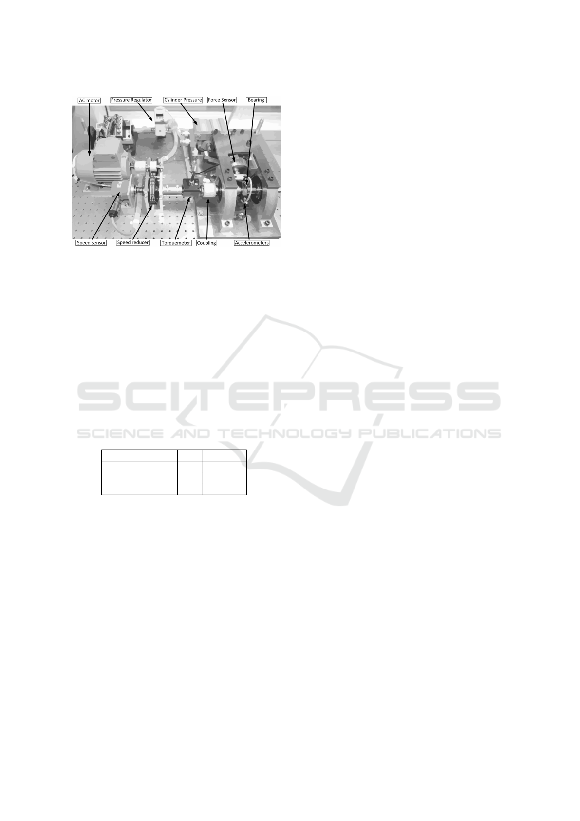
Figure 3: The Pronostia plaform.
and critical. The degradation label for each segment
is obtained by analyzing the behavior of the vibra-
tion signal. In short, the transition between regular
and degraded health stages is detected as the instant
in which the vibration results consistently equal to or
greater than 1 g (Alfeo et al., 2022). On the other
hand, the transition from the degraded to the critical
health stage is determined by looking for a sudden in-
crease in the Root Mean Square (Mao et al., 2019).
More details about this labeling procedure are pro-
vided in (Alfeo et al., 2022). As a result, each case
study results in a number of instances per degradation
stage as detailed in Table 1.
Table 1: Instances per class and case study.
Degradation stage B11 B12 B21
Regular 1871 748 753
Degraded 1665 319 371
Critical 181 73 74
Regarding the experimental setup, the autoen-
coders are characterized by a symmetric decoder and
encoder. The encoder features 4 layers made of 128,
64, 32, and 16 artificial neurons respectively. The
multimodal encoder features the same number of lay-
ers and neurons for each modality, except for the most
internal one (i.e. with 16 neurons) that is replaced
with 3 layers (made of 64, 32, and 16 neurons) shared
among the modalities. According to the current fea-
ture extraction module, the input layer of the encoder
(as well as the output layer of the decoder) varies
to fit the input length. This results in a comparable
number of trainable parameters for each autoencoder-
based feature extraction module. All of them use
mean absolute error as training loss, 128 as batch size,
Relu as activation function, and Adam as an optimiza-
tion algorithm. To provide a baseline of the recog-
nition performances, a classic feature extraction ap-
proach can be implemented, i.e. by employing a set
of largely used ”heuristic-based” features for indus-
trial assets’ degradation analysis (Hamadache et al.,
2019). Specifically:
• 90th, 75th, 50th, and 25th percentile of the time
series
• maximum, median, mean absolute deviation,
skewness of the time series
• the difference between the global (i.e. of the
whole run to failure time series) and local (i.e. of
the current time window) mean absolute deviation
• the difference between the global and local me-
dian (Alfeo et al., 2020)
• number of continuous time-intervals with values
greater than 90th, 75th, 50th, and 25th percentile
of the time series (Alfeo et al., 2020), only for the
temperature
• number of samples greater than 50% and 25%
of the maximum of the time series (Alfeo et al.,
2020), only with temperature data
• root mean square, crest factor, impulse factor,
peak to peak, entropy, kurtosis of the time series
(Hamadache et al., 2019), only for the vibration
In addition to a performance baseline, the experi-
mental comparison employs a state-of-the-art feature
learning approach, namely contrastive learning tech-
nology, as mentioned in Section 2. Its implementation
has been released by Google and made available in
September 2021 and known as Tensorflow similarity.
Tensorflow Similarity makes available a Multi-
Similarity Loss function which measures the similar-
ity, e.g. inverse of the euclidean distance, between
the representation of 3 data points in the embedding
space i.e. the anchor, the positive, and the negative.
The anchor is similar to the positive, i.e. belongs to
the same class, and is dissimilar to the negative, i.e.
another class. To achieve these results the framework
trains the network in a way that the distance between
the anchor sample and the negative sample represen-
tations is greater (and bigger than a margin m) than the
distance between the anchor and positive representa-
tions. Regarding the performance evaluation, the ex-
perimental results are presented as a 95% confidence
interval (CI) obtained via a 10-repetitions stratified
Monte Carlo cross fold validation, featuring 90% of
the data as training set and 10% as testing set. The
hardware platform used for the experiments employs
an CPU Intel Core i5-3337U@1.80GHZ, RAM 6 GB
DDR3, and an GPU Invidia GeForce GT 630M.
The considered classification problem is unbal-
anced, since the regular stage lasts longer than the
critical one and this results in less instances of the
IN4PL 2022 - 3rd International Conference on Innovative Intelligent Industrial Production and Logistics
98
more severe degradation stage. For this reason the
classification performance is measured in terms of
F1-score (Nguyen, 2019), i.e. the harmonic mean of
precision and recall, where the precision is the num-
ber of true positives divided by the number of all pos-
itives, and the recall is the number of true positives
divided by the number of all samples that should have
been identified as positive (Eq. 1). The highest possi-
ble value of an F-score is 1.0, indicating perfect pre-
cision, I.e., there are no false positives (e.g. a critical
stage recognized as a regular one), and perfect recall,
i.e. There are no false negatives (e.g. a regular stage
recognized as a critical one), the lowest possible value
for the F1-score is 0 if either the precision or the re-
call is zero, I.e., there are no true positives (e.g. a
correctly recognized regular stage).The highest possi-
ble value of an F-score is 1.0, indicating perfect pre-
cision, I.e., there are no false positives (e.g. a critical
stage recognized as a regular one), and perfect recall,
i.e. There are no false negatives (e.g. a regular stage
recognized as a critical one), the lowest possible value
for the F1-score is 0 if either the precision or the recall
is zero, I.e., there are no true positives (e.g. a correctly
recognized regular stage).For the sake of readability,
the F1-score is multiplied by 100, so that the values
would be bounded between 0 (worst case) and 100
(best case).Since the classification problem features
more than 2 classes, we consider the average of the
F1-scores for each class as the global F1-score.
F1 =
2 ∗ Precision ∗ Recall
Precision + Recall
=
2 ∗ T P
2 ∗ T P + FP + FN
(1)
A feature can be considered informative, if it ease
the separation of the instances among classes (Lorena
et al., 2019). In this regard, class separability metrics
may correlate with classification accuracy (Skrypnyk,
2011), (Cano, 2013). The class separability metrics
allows measuring how well the learned features space
helps separating different classes. In this context, the
so called L1 measure quantifies whether the classes
can be linearly separated in the feature spaces (Lorena
et al., 2019). Specifically, the L1 measure is com-
puted as the sum of the distances of incorrectly clas-
sified examples to a linear boundary used in their clas-
sification. If the value of L1 is zero, then the problem
is linearly separable and can be considered simpler
than a problem for which a non-linear boundary is re-
quired. Lower values for L1 (bounded between 0 and
1) indicate that the problem is close to being linearly
separable, thus simpler. For the sake of readability,
1 − L1 is employed as class separability metric, and
multiply it by 100, so that the values reported in this
work would be bounded between 0 (worst case) and
100 (best case). A qualitative evaluation of the class
separability is presented via a visualization of the in-
stances in the learned feature space. By being mul-
tidimensional, such feature space is almost impossi-
ble to represent graphically. Thus, the feature space
is represented via a projections over its two principal
components’ directions. Of course, such projection
is a valid tool for visualization purposes and qualita-
tive analysis, but it may not exhaustively represent the
proximity between the instances in the feature space
(Liu et al., 2021).
5 RESULTS
In the following, the different feature extraction ap-
proaches are shortened as follows: heuristic-based
features (HB), partition-based autoencoder (PAE),
shared-input autoencoder (SAE), multi-modal au-
toencoder (MMAE), similarity-based encoder (SE).
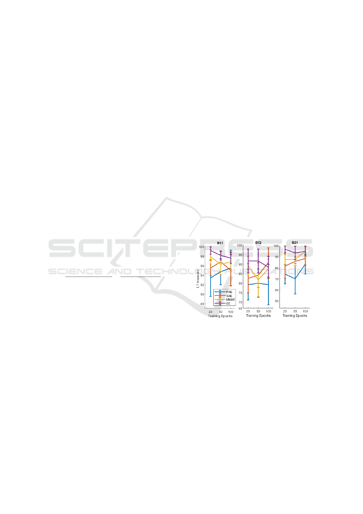
First, it is tested how training epochs impact on
the quality of features learned, which is measured in
terms of class separability with the L1 measure. Fig.
4 shows such quality as training epochs increase (i.e.,
25, 50 and 100 epochs) for each feature learning ap-
proach considered.
Figure 4: L1 measure by changing the number of training
epochs and feature extraction approach. Average and 95%
confidence interval.
The trend observed in the results is a non-
consistent and almost negligible improvement in the
class separability metric. This is also confirmed by
considering the results in terms classification perfor-
mance which are slightly better or comparable despite
the number of training epochs used. Indeed, the great-
est increase in classification performance is obtained
with SAE and the B21 case study: here increasing the
number of training epochs from 25 to 100 results in a
F1-score increase of 4.01%. By considering just the
average separability metrics, PAE seems to results in
features with the worst average class separability with
2 cases study over 3, whereas SE results in features
Automatic Feature Extraction for Bearings’ Degradation Assessment using Minimally Pre-processed Time series and Multi-modal Feature
Learning
99
with the best average class separability with 2 cases
study over 3.
Next, it is tested if the class separability obtained
with the features provided by the different Feature Ex-
traction (FE) approaches is correlated to their classi-
fication performance. Table 2 reports the the L1 mea-
sures obtained with the features provided by each FE
approach, with 100 training epochs. Moreover, Table
3 reports the F1-scores obtained with the KNN classi-
fier by using the features obtained with each Feature
Extraction (FE) approach, and 100 training epochs.
The best average performances for each case study is
highlighted in bold.
Table 2: L1 measure using 100 training epochs for each
Feature Extraction (FE) approach. Average ± 95% confi-
dence interval. 3 degradation stages. In italic the AE-based
approaches.
FE B11 B12 B21
PAE 95.79±3.79 79.17±10.61 83.33±8.89
SAE 95.26±3.30 90.83±7.67 88.33±5.76
MMAE 97.11±1.65 87.50±5.07 95.0 ± 5.03
HB 90.0 ± 4.7 67.50±23.92 80.0 ±14.11
SE 97.89±1.19 88.33±5.76 95.0 ± 4.17
Table 3: F1-score using KNN (k=1) and 100 training epochs
for each Feature Extraction (FE) approach. Average ± 95%
confidence interval. 3 degradation stages. In italic the AE-
based approaches.
FE B11 B12 B21
PAE 97.79±0.32 88.04±2.52 90.47±2.08
SAE 98.85±0.22 93.25±1.26 96.76±0.96
MMAE 98.88±0.27 91.99±1.74 96.43±0.68
HB 94.44±1.91 74.61 ± 5.2 79.31±3.81
SE 98.59±0.29 91.90±1.99 94.62 ±1.7
As shown in Table 3, all feature learning ap-
proaches offer better degradation stage recogni-
tion performance than the heuristic-based features.
Among all the variations of the feature learning mod-
ule, PAE offers the worst performance, in accordance
with the results obtained with the separability met-
rics in 2. The performances offered by the other ap-
proaches are similar. Moreover, there is a clear cor-
relation between the average separability metric ob-
tained in a given case study and the corresponding
average classification performance. For example, the
average separability metrics in case B11 are all be-
tween 90 and 97.11, and the average F1 score is be-
tween 94.44 and 98.88. In the case of B21 the average
separability metrics are clearly lower and the average
F1 score do not exceed 93.25. It is interesting to note
that SE has comparable or worse performance than
other unsupervised approaches, despite being a super-
vised approach specifically designed to separate fea-
tures of different classes in the latent space. To do so,
SE employs a much more complex training process,
resulting in way longer training time, as confirmed by
the training times of the various feature learning mod-
ules(Table 4). Besides SE, PAE has a longer training
time because it has to be trained for each modality,
whereas SAE and MMAE require only one training
procedure. The further difference between MMAE
and SAE can be motivated by considering that, with
a fully connected neural network, an input twice as
long corresponds to a neural network input layer fea-
turing twice as many connections between neurons,
that are the actual parameters to train in a neural net-
work. Considering the number of input sensors ( i.e.
the number of modalities ) as a variable for the train-
ing time computation it can be seen that SAE, MMAE
and SE need a single training phase to handle all the
modalities at the same time, PAE instead needs to
train one AE for each modality resulting in bigger
compressive training time as table 4 shows.
Table 4: Training time [s] of each trainable Feature Extrac-
tion (FE) module. Average ± 95% confidence interval. 3
degradation stages. In italic the AE-based approaches.
FE B11 B12 B21
PAE 82.27±1.77 51.60±1.79 54.07±1.84
SAE 42.95±3.08 28.90±5.64 28.71±1.98
MMAE 42.76±4.11 22.01±0.43 22.10±1.32
SE 652.62±90.7 582.66±19.7 585.64±12.2
The results suggest that both the feature learning
module based on MMAE and SAE are the most con-
venient for the proposed 3-stages classification prob-
lem. The goodness of the proposed approach is also
tested with a more complex classification problem,
e.g., with a higher number of degradation stages to
consider. For this experimentation different degrada-
tion stages are considered, i.e. the time intervals in
which the bearing is in degradation stages ”regular”
and ”degraded” are splitted (in half) into new degra-
dation stages. The resulting problem is a five-stages
bearing degradation recognition. Table 5 reports the
classification performance obtained with each varia-
tion of the proposed approach, as well as the ones ob-
tained with the heuristic-based feature.
The classification performance obtained by using
the heuristic-based features are dramatically lower
compared to the ones obtained with 3 degradation
stages. This may be not only due to the higher com-
plexity of the classification task but also due to the
fact that both the split among the 3 degradation stages
and the heuristic-based features are specifically de-
signed to represent some physical characteristics of
the degradation phenomenon. Instead, the degrada-
IN4PL 2022 - 3rd International Conference on Innovative Intelligent Industrial Production and Logistics
100
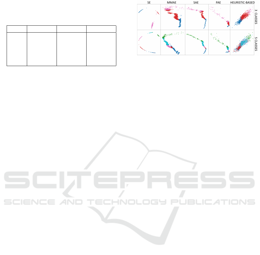
Table 5: F1-score with KNN (k=1) and 100 training epochs
for each Feature Extraction (FE) approach. Average ± 95%
confidence interval. 5 degradation stages. In italic the AE-
based approaches.
FE B11 B12 B21
PAE 92.93±1.06 80.81±4.06 80.06±2.51
SAE 97.06 ± 0.5 88.53±1.56 88.97±2.27
MMAE 97.10±0.74 87.90±1.48 90.11±1.07
HB 50.59±3.62 37.11±4.75 39.66±6.87
SE 95.89±0.98 86.08±1.88 86.24±2.89
tion stages of the 5-stages classification problem are
partially arbitrary. All the approaches based on fea-
ture learning provide average classification perfor-
mances greater than 90 with case study B11, and
greater than 80 with the others. Also in this case
the classification performance of PAE is the worst
among all the feature learning approaches. On the
contrary, MMAE and SAE provide the best classifica-
tion performances in all 3 case studies, despite provid-
ing lower performances that the ones obtained with
the 3-stages classification problem.
Fig. 5 provides a qualitative assessment of how
easily the classes can be distinguished by projecting
the obtained features onto their 2 principal compo-
nents. In this regard, even if the samples correspond-
ing to more severe degradation stages are arranged
progressively, with the heuristic-based features the
samples of different classes seems to be projected
pretty close with each others. This partially explain
the poor classification performances, especially in the
5-stages classification problem. On the other hand,
feature learning approaches result in clearly separa-
ble and adjacent group of samples corresponding to
more severe degradation stages. This simplifies the
classification task even when performed with really
simple approaches like KNN with 1 neighbor. Inter-
estingly, this property seems to be maintained even in
the 5-stages classification problem, and thus support
the good recognition performance obtained in such a
classification task.
The obtained results confirm how those feature
learning approaches succeed in capturing the progres-
sion of the degradation phenomenon, despite being
trained in an unsupervised manner, and regardless of
the number of degradation stages, as well as their ar-
rangement over time.
6 CONCLUSION
This work proposes an architecture based on au-
toencoders to automatically extract degradation-
representative features from minimally preprocessed
Figure 5: Features learned with the B11 test samples and
projected over two Principal Components. The degradation
stages ranges from regular (blue) to critical (pink with 3
classes, green with 5 classes).
time series of vibration and temperature of indus-
trial bearing. By using a publicly available real-world
dataset about bearings’ progressive degradation to test
the proposed approach against manual feature ex-
traction and the state-of-the-art technology in feature
learning. According to the obtained results, the au-
toencoders featuring a data fusion mechanism at data-
and architecture-level (i.e. SAE and MMAE) result
in features characterized by greater quality. Indeed,
those provide easily separable classes in the space of
learned features, and thus are able to simplify the clas-
sification task even if performed via simple classifica-
tion approaches, i.e. via a KNN classifier considering
just one neighbor.
Compared with manually extracted features, the
proposed approach results an increase of the classifi-
cation performances up to 19%. At the same time, by
being data-driven, the proposed approach does not re-
quire any effort to choose and design the features to
be extracted from the input data. In this work, a min-
imalist preprocessing procedure is proposed; it con-
sists of a frequency domain transformation for only
the vibration time series, and a subsequent window
aggregation of the resulting vectors. This input for-
mat, passed to each of the feature learning approaches
tested, produced features that allow clear separation
of classes, as qualitatively confirmed by the projec-
tions of the samples onto the principal components of
the feature space.
Interestingly, the multimodal autoencoder results
in recognition performances that are comparable with
the ones obtained via state-of-the-art approaches (i.e.
based on contrastive learning) despite being trained in
an unsupervised manner, and regardless of the num-
ber of degradation stages considered.
The promising results provided in this study leave
room for more intensive experimentation as the num-
ber and type of input modalities vary. As future
works, more recent datasets and better-performing
methods than KNN can be used to further test the
proposed approach and improve recognition perfor-
Automatic Feature Extraction for Bearings’ Degradation Assessment using Minimally Pre-processed Time series and Multi-modal Feature
Learning
101

mance. Moreover, assets’ degradation can be mon-
itored with measures such as acoustic noise, power
consumption, torque and many more. By including
all these modalities, it would be possible to test the ca-
pacity of the proposed approach to be data-agnostic,
that is, valid regardless of the measure used to assess
the current degradation stage.
ACKNOWLEDGEMENTS
Work partially supported by (i) the Tuscany Region
in the framework of the SecureB2C project, POR
FESR 2014-2020, Project number 7429 31.05.2017,
(ii) the Italian Ministry of University and Research
(MUR), in the framework of the ”Reasoning” project,
PRIN 2020 LS Programme, Project number 2493 04-
11-2021, and (iii) the Italian Ministry of Education
and Research (MIUR) in the framework of the Cross-
Lab project (Departments of Excellence). The authors
thank Mario Alberto Gherardi for his work on the sub-
ject during his master thesis.
REFERENCES
Alfeo, A. L., Cimino, M. G., Manco, G., Ritacco, E., and
Vaglini, G. (2020). Using an autoencoder in the de-
sign of an anomaly detector for smart manufacturing.
Pattern Recognition Letters, 136:272–278.
Alfeo, A. L., Cimino, M. G., and Vaglini, G. (2021). Tech-
nological troubleshooting based on sentence embed-
ding with deep transformers. Journal of Intelligent
Manufacturing, 32(6):1699–1710.
Alfeo, A. L., Cimino, M. G., and Vaglini, G. (2022). Degra-
dation stage classification via interpretable feature
learning. Journal of Manufacturing Systems, 62:972–
983.
Bengio, Y., Courville, A., and Vincent, P. (2013). Represen-
tation learning: A review and new perspectives. IEEE
transactions on pattern analysis and machine intelli-
gence, 35:1798–1828.
Cano, J.-R. (2013). Analysis of data complexity measures
for classification. Expert systems with applications,
40(12):4820–4831.
Deng, L. (2014). A tutorial survey of architectures, algo-
rithms, and applications for deep learning. APSIPA
transactions on Signal and Information Processing, 3.
Elie Bursztein, James Long, S. L. O. V. F. C. (2021). Ten-
sorflow similarity: A usable, high-performance metric
learning library. Fixme.
Gao, J., Li, P., Chen, Z., and Zhang, J. (2020). A survey
on deep learning for multimodal data fusion. Neural
Computation, 32(5):829–864.
Gecgel, O., Ekwaro-Osire, S., Gulbulak, U., and Morais,
T. S. (2022). Deep convolutional neural network
framework for diagnostics of planetary gearboxes un-
der dynamic loading with feature-level data fusion.
Journal of Vibration and Acoustics, 144(3).
Hamadache, M., Jung, J. H., Park, J., and Youn,
B. D. (2019). A comprehensive review of artifi-
cial intelligence-based approaches for rolling element
bearing phm: shallow and deep learning. JMST Ad-
vances, 1(1):125–151.
Jimenez, J. J. M., Schwartz, S., Vingerhoeds, R., Grabot,
B., and Sala
¨
un, M. (2020). Towards multi-model ap-
proaches to predictive maintenance: A systematic lit-
erature survey on diagnostics and prognostics. Journal
of Manufacturing Systems, 56:539–557.
Kimotho, J. K., Sondermann-W
¨
olke, C., Meyer, T., and
Sextro, W. (2013). Machinery prognostic method
based on multi-class support vector machines and hy-
brid differential evolution–particle swarm optimiza-
tion. Chemical Engineering Transactions, 33.
Lei, Y., Li, N., Guo, L., Li, N., Yan, T., and Lin, J. (2018).
Machinery health prognostics: A systematic review
from data acquisition to rul prediction. Mechanical
systems and signal processing, 104:799–834.
Liu, Y., Hu, Z., and Zhang, Y. (2021). Bearing feature
extraction using multi-structure locally linear embed-
ding. Neurocomputing, 428:280–290.
Lorena, A. C., Garcia, L. P., Lehmann, J., Souto, M. C., and
Ho, T. K. (2019). How complex is your classification
problem? a survey on measuring classification com-
plexity. ACM Computing Surveys (CSUR), 52(5):1–
34.
Mao, W., He, J., and Zuo, M. J. (2019). Predicting re-
maining useful life of rolling bearings based on deep
feature representation and transfer learning. IEEE
Transactions on Instrumentation and Measurement,
69(4):1594–1608.
Merkt, O. (2019). Predictive models for maintenance opti-
mization: an analytical literature survey of industrial
maintenance strategies. Information Technology for
Management: Current Research and Future Direc-
tions, pages 135–154.
Nectoux, P., Gouriveau, R., Medjaher, K., Ramasso, E.,
Chebel-Morello, B., Zerhouni, N., and Varnier, C.
(2012). Pronostia: An experimental platform for bear-
ings accelerated degradation tests. In IEEE Interna-
tional Conference on Prognostics and Health Man-
agement, PHM’12., pages 1–8. IEEE Catalog Num-
ber: CPF12PHM-CDR.
Nelli, F. (2018). Machine learning with scikit-learn. In
Python Data Analytics, pages 313–347. Springer.
Ngiam, J., Khosla, A., Kim, M., Nam, J., Lee, H., and Ng,
A. Y. (2011). Multimodal deep learning. In ICML.
Nguyen, M. H. (2019). Impacts of unbalanced test data
on the evaluation of classification methods. Recall,
100:90–00.
Pandarakone, S. E., Masuko, M., Mizuno, Y., and Naka-
mura, H. (2018). Deep neural network based bearing
fault diagnosis of induction motor using fast fourier
transform analysis. In 2018 IEEE energy conversion
congress and exposition (ECCE), pages 3214–3221.
IEEE.
IN4PL 2022 - 3rd International Conference on Innovative Intelligent Industrial Production and Logistics
102

Parola, M., Galatolo, F. A., Torzoni, M., Cimino, M., and
Vaglini, G. (2022). Structural damage localization via
deep learning and iot enabled digital twin. In Proc.
of third International Conf. on Deep Learning Theory
and Applications, July 2022, Lisbon, Portugal.
Ran, Y., Zhou, X., Lin, P., Wen, Y., and Deng, R. (2019). A
survey of predictive maintenance: Systems, purposes
and approaches. arXiv preprint arXiv:1912.07383.
Scanlon, P., Kavanagh, D. F., and Boland, F. M. (2012).
Residual life prediction of rotating machines using
acoustic noise signals. IEEE Transactions on Instru-
mentation and Measurement, 62:95–108.
Shin, B., Lee, J., Han, S., and Park, C.-S. (2021). A study
of anomaly detection for ict infrastructure using con-
ditional multimodal autoencoder. Journal of Intelli-
gence and Information Systems, 27(3):57–73.
Skrypnyk, I. (2011). Irrelevant features, class separability,
and complexity of classification problems. In 2011
IEEE 23rd International Conference on Tools with Ar-
tificial Intelligence, pages 998–1003. IEEE.
Tang, S., Yuan, S., and Zhu, Y. (2019). Deep learning-
based intelligent fault diagnosis methods toward ro-
tating machinery. Ieee Access, 8:9335–9346.
Vincent, P., Larochelle, H., Lajoie, I., Bengio, Y., Man-
zagol, P.-A., and Bottou, L. (2010). Stacked denois-
ing autoencoders: Learning useful representations in a
deep network with a local denoising criterion. Journal
of machine learning research, 11.
Vinh, N. X., Epps, J., and Bailey, J. (2009). Information the-
oretic measures for clusterings comparison: is a cor-
rection for chance necessary? pages 1073–1080.
Wan, J., Tang, S., Li, D., Wang, S., Liu, C., Abbas, H., and
Vasilakos, A. V. (2017). A manufacturing big data so-
lution for active preventive maintenance. IEEE Trans-
actions on Industrial Informatics, 13:2039–2047.
Yan, W. and Yu, L. (2015). On accurate and reliable
anomaly detection for gas turbine combustors: A deep
learning approach. In Annual Conference of the PHM
Society, volume 7.
Yan, X., Liu, Y., and Jia, M. (2020). Health condition
identification for rolling bearing using a multi-domain
indicator-based optimized stacked denoising autoen-
coder. Structural Health Monitoring, 19:1602–1626.
Zhong, G., Ling, X., and Wang, L.-N. (2019). From shal-
low feature learning to deep learning: Benefits from
the width and depth of deep architectures. Wiley In-
terdisciplinary Reviews: Data Mining and Knowledge
Discovery, 9:e1255.
Automatic Feature Extraction for Bearings’ Degradation Assessment using Minimally Pre-processed Time series and Multi-modal Feature
Learning
103
