
Deep Learning of Structural Changes in Historical Buildings: The Case
Study of the Pisa Tower
Mario G. C. A. Cimino
1 a
, Federico A. Galatolo
1 b
, Marco Parola
1 c
,
Nicola Perilli
2
and Nunziante Squeglia
2 d
1
Dept. of Information Engineering, University of Pisa, 56122 Pisa, Italy
2
Dept. of Civil and Industrial Engineering, University of Pisa, 56122 Pisa, Italy
Keywords:
Structural Health Monitoring, Multi-sensor System, Transformer, LSTM, Leaning Tower of Pisa.
Abstract:
Structural health monitoring of buildings via agnostic approaches is a research challenge. However, due to the
recent advent of pervasive multi-sensor systems, historical data samples are still limited. Consequently, data-
driven methods are often unfeasible for long-term assessment. Nevertheless, some famous historical buildings
have been subject to monitoring for decades, before the development of smart sensors and Deep Learning
(DL). This paper presents a DL approach for the agnostic assessment of structural changes. The proposed
approach has been experimented to the stabilizing intervention carried out in 2000-2002 on the leaning tower
of Pisa (Italy). The data set is made by operational and environmental measures collected from 1993 to 2006.
Both conventional and recent approaches are compared: Multiple Linear regression, LSTM and Tansformer.
Experimental results are promising, and clearly shows a better change sensitivity of the LSTM, as well as a
better modeling accuracy of the Transformer.
1 INTRODUCTION
Structural health monitoring (SHM) plays an impor-
tant role in the diagnosis and evaluation of the sta-
bility and deformation of historical buildings. Over
the ages, such buildings have been subject to various
maintenance and renovations, using different materi-
als and construction techniques, leading to a complex
structural behavior.
Multi-sensor systems with high reliability and low
cost, small size and weight, low power consumption
and high rate data processing, are essential to SHM.
However, their pervasive application is still in its in-
fancy. As a consequence, long-term data are available
only for world famous historical buildings. For such
buildings, sensor systems gathering multiple parame-
ters for long time allow the experimentation of agnos-
tic techniques based on Deep Learning (DL) (Farrar
et al., 2006).
In the literature, according to the type of param-
eters acquired, SHM systems are classified into two
a
https://orcid.org/0000-0002-1031-1959
b
https://orcid.org/0000-0001-7193-3754
c
https://orcid.org/0000-0003-4871-4902
d
https://orcid.org/0000-0001-8104-503X
main categories: (i) static systems, which monitor the
temporal evolution of quantities that change slowly
over time (e.g., crack widths, wall slopes, relative dis-
tances, etc.) via periodic data sampling; (ii) dynamic
systems, which monitor dynamic parameters such as
velocities, accelerations, in order to gather informa-
tion on general dynamic properties such as natural
frequencies, mode shapes, and damping ratios.
Data pre-processing is also essential, because dif-
ferent sensing technologies can be employed over the
ages, as well as to distinguish any evolutionary trends
from seasonal and daily variations related to environ-
mental effects (Baraccani et al., 2017).
As a methodology of data analysis for SHM, DL
techniques have shown a significant potential for their
capabilities of detecting implicit relationships in data,
by requiring less domain knowledge. Some DL archi-
tectures have been already experimented for specific
tasks on particular buildings (Mishra, 2021); e.g. a
convolutional architecture to solve the damage local-
ization task (Parola. et al., 2022). A relevant state-of-
the art review is provided in next section.
In this paper, the Transformer architecture is pro-
posed and compared with the Long-Short Term Mem-
ory (LSTM) for a specific SHM task. In the lit-
erature, it is well-known that a Transformer over-
396
Cimino, M., Galatolo, F., Parola, M., Perilli, N. and Squeglia, N.
Deep Learning of Structural Changes in Historical Buildings: The Case Study of the Pisa Tower.
DOI: 10.5220/0011551800003332
In Proceedings of the 14th International Joint Conference on Computational Intelligence (IJCCI 2022), pages 396-403
ISBN: 978-989-758-611-8; ISSN: 2184-3236
Copyright © 2023 by SCITEPRESS – Science and Technology Publications, Lda. Under CC license (CC BY-NC-ND 4.0)

come an LSTM in the semantic capture of time-series
data. The different solutions are compared in order to
asses the structural changes in the Leaning Tower of
Pisa (Italy) (Burland et al., 2009), which has under-
gone many maintenance intervention over the epochs.
Specifically, the under-excavation intervention per-
formed between 2000 and 2001 is considered (Bur-
land et al., 2009) as a case study.
The SHM system installed on the Leaning Tower
of Pisa is a static system, with a configurable sam-
pling time period. Figure 1 shows some sensing sub-
systems installed inside the tower since 1993, deliver-
ing a synchronized Multivariate Time Series (MTS).
The data series hourly collected from 1993 to
2006, has been used for the assessment of the above
mentioned under-excavation effects, via both conven-
tional and recent approaches: Multiple Linear Regres-
sion, LSTM and Transformer.
The underlying strategy for the proposed approach
is to create a model of the structural behavior before
and after the maintenance intervention, exploiting the
large availability of data, via a general purpose pre-
processing, and without a knowledge-based supervi-
sion nor feature selection. This approach falls under
the regression task, whose goal is the agnostic model
of the relationship between input and output data. In
particular, prediction is a special type of regression
aimed to foresee the next values of a given time se-
ries. In the proposed approach, a multi input - multi
output prediction is considered.
(a)
(b)
(c)
Figure 1: Some sensing subsystems of the tower of Pisa:
(a) telecoordinometer - inclinometer and pendulum; (b) en-
vironmental parameters - wind speed and direction, solar
radiation and termometer; (c) deformometer.
Finally, the assessment of the structural change is
based on the differences in the prediction capability
of the model before and after the maintenance event.
Experimental results are promising, and clearly shows
the higher accuracy of Transformer, with respect to
LSTM and conventional Multi-Linear Regression, as
well as the better sensitivity of LSTM.
The paper is structured as follows. Section 2
presents an overview of the related works. Section
3 covers material and methods, whereas experimen-
tal results and discussions are covered by Section 4.
Finally, Section 5 draws conclusions and future work.
2 RELATED WORKS
A structural change of a building is measured via a
change of the materials and/or physical properties of
the structure. For example, an elastic material coef-
ficient reduction and system connectivity, which ad-
versely affect the system’s current or future perfor-
mance (Farrar and Worden, 2007).
In the literature, the structural changes of a main-
tenance intervention can be detected via a two-phase
method: (a) to identify the stable key parameters of
a behavioral model of the structure, corresponding to
the periods before and after the intervention; (b) to
identify a persistent variation of such parameters by
comparing the two periods. The underlying idea is
that a change of behavior on the structure will occur
over time after the intervention in terms of deviation
from the condition before the intervention (Reynders
et al., 2014).
The main drawback of this approach is the knowl-
edge needed to set up a model, the key parameters,
and the baseline condition representing the state be-
fore the maintenance. A possible solution is to ex-
ploit multivariate clustering in feature space for the
identification of the stable clusters/components that
describe the behavior of the structure (Figueiredo
et al., 2014). An alternative approach, requiring lit-
tle knowledge, is to exploit regression analysis, where
both environmental and operational properties are
taken into account to generate a predictive model of
the behavior before the maintenance, which can be
used for the behavior after the maintenance, in order
to assess a different deviation from the expected value
(Wah et al., 2021).
In this work, a regression-based approach is pro-
posed, by using the data provided by the multi-sensor
system in order to model the related Multivariate
Time Series (MTS). A MTS represents the evolution
of a group of variables partially independent. The pre-
diction of a MTS can be solved via a classical statis-
tical approach, such as an auto-regressive integrated
moving average method, which can be used to ana-
lyze the relationships between the different variables.
In the last decade, DL-based methods achieved
Deep Learning of Structural Changes in Historical Buildings: The Case Study of the Pisa Tower
397
widespread adoption, for their effectiveness. Dif-
ferent architectures have been experimented to solve
the MTS prediction problem, such as Recurrent Neu-
ral Network (RNN), Gated Recurrent Unit (GRU)
or Long short-term memory (LSTM). More recently,
Transformer have shown to perform better on both
synthetic and real datasets, due to their attention
mechanism (Li et al., 2019). In this research, both
conventional and recent approaches are compared:
Multiple Linear regression, LSTM and Tansformer.
3 MATERIALS AND METHODS
This section covers, on different subsections, the
multi-sensor system providing the MTS, the pre-
processing of the MTS samples, as well as the regres-
sion models adopted for MTS prediction.
3.1 Multi-sensor System and Data
Preprocessing
A complex system consisting of over 60 sensors is
available for the leaning tower of Pisa. In this re-
search, only a subsystem of sensors are considered to
address the structural change assessment occurred in
2000-2001. Such subsystem is defined in Table 1: (i)
operational sensors, made of 25 deformometers and 2
telecoordinometers, which measure the physical con-
dition of the tower, such as rotations or displacements;
(ii) environmental sensors, which measure the exter-
nal conditions, such as temperature, wind, solar radia-
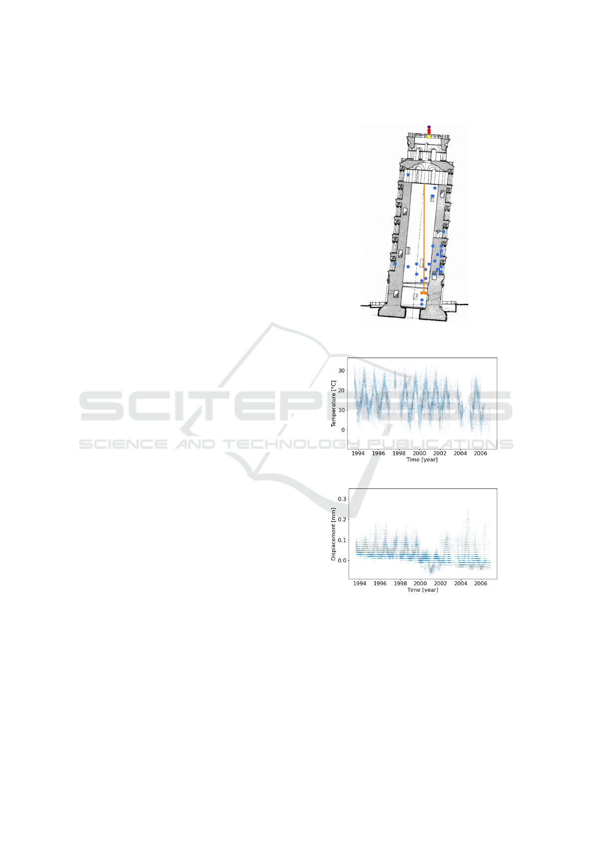
tion. Figure 2 shows the position on the tower of each
sensor. In particular, the most of the deformometers
(blue circles) are placed on the inclination side, on
bottom-right in figure, where the high load / stress is
located. Environmental sensors (yellow, red and pur-
ple circles) are placed on the top. Finally, the orange
long plumb wire of the telecoordinometer is clearly
visible in the middle.
Figure 3 and Figure 4 show a global plot over 13
years of the temperature and a deformometer time se-
ries. Series of samples related to very long periods
are normally affected by different artifacts: outliers,
missing samples, sensors re-calibration, sensors hard-
ware replacement/maintenance, and so on. As a con-
sequence, data preprocessing is of the utmost impor-
tance to avoid biases and false positives. Specifically,
outliers are due to electronic devices errors, which are
sometimes affected by sensor reading issues, resulting
in out-of-scale samples. On the other side, missing
data samples are due to hardware, power or network,
failures that sometimes occur. Finally, hardware re-
placement, maintenance and recalibration cause scal-
ing artifacts.
Figure 2: Multi-sensor system distribution on the tower, ac-
cording to the color legend in Table 1.
Figure 3: Global plot on 13 years of the temperature series.
Figure 4: Global plot on 13 years of a deformometer series.
The pre-processing pipeline is made by different
tasks:
1. out-of scale outliers detection, on the basis of
lower and upper thresholds;
2. z-score normalization, to reduce artifacts related
to scaling. Equations (1) shows the formula of the
z-score. Given a signal x = [x
1
, ..., x
n
], the nor-
malized signal z can be computed by subtracting
NCTA 2022 - 14th International Conference on Neural Computation Theory and Applications
398

from each element the mean value ¯µ
i
computed
on all elements as shown in Equation (2) and di-
viding by their standard deviation
¯
σ
i
as shown in
Equation (3);
3. statistical outliers detection, in which samples
having value of ±3 farther from the current mov-
ing average (window size, w=100) are selected;
4. outliers/ isolated missing samples reconstruction,
in which a linear interpolation between the near-
est neighbors is carried out for the outliers previ-
ously determined, and short sequences of consec-
utive missing samples (at most 4 elements). Long
sequences of missing values, e.g. due to device
failure, are not reconstructed at all.
5. hourly data resampling. Figure 5 shows a two-
weeks plot of a deformometer time series. During
the considered period, as a consequence of main-
tenance, some changes in the frequency of device
reading activation occurred. To remove this type
of artifact, the entire time series is resampled with
one hour frequency.
z
i
=
x
i
− ¯µ
i
¯
σ
i
(1)
¯µ
i
=
∑
i−1
j=i−w
x
j
w
(2)
¯
σ
i
=
s
∑
i−1
j=i−w
(x
i
− x
j
)
2
w
(3)
Figure 5: Two-weeks plot of a deformometer time series.
Figure 6 shows the distribution of samples for
each sensor in the considered period of observation,
separated in pre-maintenance (blue circles) and post-
maintenance (orange circles). Here, according to Ta-
ble 1, each sensor is identified by a letter and an in-
cremental number.
It is clear from the figure that the two distributions
highly overlap. As a consequence, statistical or data
mining approaches to structural change detection are
human knowledge driven. As a consequence, in this
paper, agnostic regression-based methodologies will
be applied and compared.
3.2 Multivariate Linear Regression
Model and Performance Metrics
In the proposed regression approach to structural
changes assessment three data sets are first created:
1. pre-maintenance set (pre for short);
2. post-maintenance set (post);
3. pre- and post- maintenance (full).
Table 1: Subsystem of sensors installed on the leaning tower and used for the proposed research.
Sensor # Leg Thresholds Description
Deformometer (D) 25 [-0.5,0.5] mm Detects dimensional deformations of a struc-
ture subjected to mechanical or thermal
stresses.
Telecoordinometer (T) 2 [-2100,1800] ” Measures a small rotation by reading the posi-
tion of a plumb wire.
Termometer (TM) 1 [-10,42] °C Measures the atmospheric temperature.
Wind speed sensor (WS) 1 [0,45] m/s Measures wind speed; the wind drives the top
three wind cups to rotate, and the central axis
drives the sensing element to generate an output
used to calculate the wind speed.
Wind direction sensor (WD) 1 [0,360] degree Measure wind direction; it works through the
rotation of a wind vane arrow and transmits
its measurement information to the coaxial en-
coder board.
Solar radiation sensor (SR) 1 [0,1000] W/m
2
Measure broadband solar irradiance by detect-
ing the photons that impact a physical or chem-
ical device located within the instrument.
Deep Learning of Structural Changes in Historical Buildings: The Case Study of the Pisa Tower
399

Figure 6: Values distribution (y-axis) for each separate sensor (x-asis), in the pre- and post- maintenance periods.
Specifically, the intervals of the pre, post and full
periods are, respectively: [Aug 1st, 1993 - Aug 31,
1999], [Jan 01, 2002 - Jun 30, 2006], [Jan, 08, 1993 -
June 30, 2006]. Then, three different prediction mod-
els are generated, using related subsets of the pre, post
and full sets, respectively, for training. Subsequently,
the generated models are tested on other subsets of
the pre, post and full sets.
Since a predictive model can be tested only on
future samples, there are four possible experiments
based on a combination of train and test sets: (a) full-
full; (b) pre-pre; (c) post-post; (d) pre-post.
Finally, the structural change assessment is carried
out by evaluating the difference in test performance
between the four experiments: roughly speaking, if
the test error is higher for the pre-post experiment
with respect to the other experiments, it means that
the model generated in the pre-maintenance period is
unable to accurately predict the behavior in the post-
maintenance period; and then, a structural change has
occurred between pre and post periods; otherwise, if
the error for the pre-post experiment is similar to the
others, no structural change has occurred.
More formally, let us consider a set of n synchro-
nized time series, X(t) = {X
j
(t) : j = 1, ..., n}, where
X
j
(t) is a time series of length m, X
j
(t) = {x
j
(t) : j =
1, ..., n; t = 1, ..., m}. An MTS predictive model takes
as an input a time window w extracted from the series,
X
w
(
¯
t) = {x
w j
(t) : j = 1, ..., n; t =
¯
t, ...,
¯
t +w}, and pre-
dicts the next sample as an output The model can be
formally described by a function f : R
n×m
→ R
n×m
:
f (X
w
(
¯
t)) = X
w
(
¯
t + 1) (4)
where X
w
(
¯
t + 1) = {x
w j
(t) : j = 1, ..., n; t =
¯
t +
1, ...,
¯
t + w + 1}.
A conventional machine learning method to per-
form this task is to calculate a Multivariate Linear
Regression, whose training is based on coefficients
α
i j
and β
j
that are determined with n+1 equations, by
minimizing the error function via partial derivatives:
x
w j
(
¯
t + 1) =
n
∑
j=1
¯
t
∑
i=
¯
t
α
i j
x
w j
(i) + β
j
x
w j
(
¯
t + 2) =
n
∑
j=1
¯
t+1
∑
i=
¯
t
α
i j
x
w j
(i) + β
j
...
x
w j
(
¯
t + w + 1) =
n
∑
j=1
¯
t+w
∑
i=
¯
t
α
i j
x
w j
(i) + β
j
(5)
Given the set S of time series of length m, each
related to n sensors, in order to evaluate the model
error, trained and tested on related sets Tr ∈ S
and T s ∈ S, the overall forecasting performance is
measured via the Mean Relative Percent Difference,
MRPD(Tr; T s), i.e., the mean value of the Rela-
tive Percent Differences of each sensor (Botchkarev,
2018):
MRPD
S
(Tr; T s) =
1
n
∑
s∈S
RPD
s
(Tr; T s) (6)
The Relative Percent Difference between two values
is the absolute difference between the two values di-
vided by their absolute mean:
RPD
s
(Tr; T s) =
2
m
m
∑
k=1
|y
ks
− ¯y
ks
|
|y
ks
| + | ¯y
ks
|
; y
ks
∈ T s
(7)
The aggregation in Formula (6) of different types
of sensors via the mean operator can be done under
the assumptions that the data follow a Gaussian dis-
tribution and are also normalized. For the data sets
used in this paper, this assumption is verified via a
Q Q plot, and via the z-score normalization applied
in the pre-processing phase, respectively.
Finally, by having the accuracy values of the pre-
dictive models via MRPD
S
(Tr; T s) on the test dataset,
NCTA 2022 - 14th International Conference on Neural Computation Theory and Applications
400

the following metric of structural change assessment
(SCA) can be derived:
SCA
S
(pre; post) =
2 · MRPD
S
(pre; post)
MRPD
S
(pre; pre)· MRPD
S
(post; post)
(8)
Assuming a good accuracy of the model on the
same period, the larger SCA is, the more the structural
behavior change assessment between pre and post pe-
riods is larger. Because if the model of the pre period
does not fit the post period, the difference at the nu-
merator in Formula (8) is large with respect to the ac-
curacy at the denominator. In contrast, a small value
of the metric corresponds to a low structural change
assessment.
3.3 Deep Learning Models
Two DL models have been experimented to perform
the MTS regression task: (i) a Long-Short Term
Memory (LSTM) neural network, and (ii) a Trans-
former. The hyperparameters of the two models have
been set via grid-search, with intervals established to
keep a good accuracy and convergence. Table 2 and
Table 3 summarizes the search space and the optimal
values for each hyperparameter.
Table 2: LSTM hyperparameters optimization.
Hyperparameters
Search space Optimum
Layers [1,2,3] 2
Units [32,64,128, 256] 128
Linear layer - 31
Table 3: Transformer hyperparameters optimization.
Hyperparameters
Search space Optimum
Embedding type - Abs pos enc
Attention Head [4,5,6,7,8] 6
Layers per Head [5,6,7,8,9] 8
Neurons per layer [32,64,128] 128
In terms of parametric complexity, the Multivari-
ate Linear Regression (MLR) defined in the previ-
ous section has 70 thousand trainable parameters. An
LSTM model is designed to overcome the explod-
ing/vanishing gradient problems that typically occur
when using too many layers (Van Houdt et al., 2020).
A common LSTM unit is composed of a cell that
remembers values over arbitrary time intervals and
three gate: an input gate, an output gate and a for-
get gate, which regulate the flow of information into
and out of the cell. To model long-short term rela-
tionships, LSTM have a fairly complex internal struc-
ture, although it has been shown that similar but sim-
pler networks can achieve similar performance (Gala-
tolo et al., 2018). The LSTM architecture used has
210 thousand trainable parameters. Finally, a Causal
Transformer is a DL architecture that does not pro-
cess data in an ordered sequence, but analyzes the
entire sequence of data and exploits a self-attention
mechanisms to learn dependencies in the sequence,
achieving the potential of modeling complex dynam-
ics of time series (Vaswani et al., 2017). The Trans-
former architecture significantly exceeds the other ar-
chitectures in terms of number of trainable parame-
ters: about 2.5 million.
The training process of both LSTM and Trans-
former has been performed for 2500 epochs, with
batch size 32, by setting the Adaptive Moment Es-
timation (Adam) as optimization algorithm to itera-
tively update the network weights.
4 EXPERIMENTAL RESULTS
The methodology has been developed on a python
open-source environment, which has been publicly
released (Galatolo, 2022), to foster collaboration and
application on various infrastructures. This section
summarizes and discusses the experimental results
achieved with the three considered architectures. To
this aim, Table 4 illustrates the results of the predic-
tion models. In particular, the MRPD is computed
aggregating each type of operational sensor (average
± standard deviation): 25 Deformometers (D*) or 2
Telecoordinometer (T*). Envirnomental sensors are
not considered as an output because they are not re-
lated to structural changes but to environmental vari-
ations.
Let us consider test performance, i.e.,
MRPD
D∗
test and MRPD
T ∗
test columns. In par-
ticular, let us focus on the values represented in
boldface style, i.e., the test performance on pre
and post sets for train and test, respectively. It can
be clearly observed that DL models, i.e., LSTM
and TRANS, perform better than MLR in pre-post
prediction, with LSTM model achieving the highest
score (.814 and 1.407). Furthermore, DL models are
more accurate in pre-pre and post-post prediction,
by having a lower score, especially TRANS model
(.256, .324 and .119, .145). Overall, TRANS is the
most accurate model whereas LSTM is the most
sensitive model to structural changes.
In order to analyze the contribution of each sen-
sor to the result, in Figure 7, the RPD value with
the related standard deviation on test set is repre-
sented, as a coloured circle with a vertical line, re-
spectively, for each DL model. Here, a horizontal red
line represents the MRPD already calculated in Table
Deep Learning of Structural Changes in Historical Buildings: The Case Study of the Pisa Tower
401
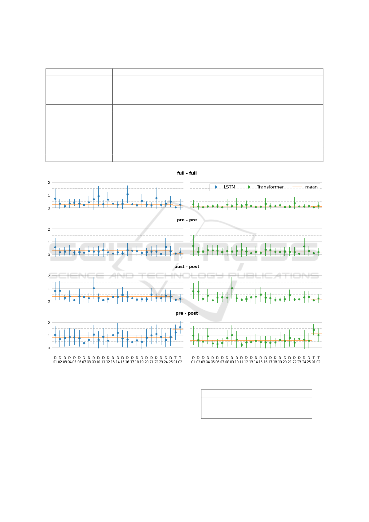
Table 4: MRPD on train and test set, for different models, using Deformometers (D*) or Telecoordinometers (T*) time series.
Model Train Test MRPD
D∗
train MRPD
D∗
test MRPD
T ∗
train MRPD
T ∗
test
MLR full full .234 ±.0081 .221 ±.0065 .276 ±.0068 .398 ±.0068
” pre pre .406 ±.0117 .435 ±.0114 .378 ±.0076 .277 ±.0072
” post post .393 ±.103 .434 ±.0118 .257 ±.0057 .212 ±.0041
” pre post .406 ±.0117 .522 ±.0122 .378 ±.0076 .605 ±.0161
TRANS full full .124 ±.0052 .141 ±.0050 .055 ±.0032 .112 ±.0038
” pre pre .219 ±.0077 .256 ±.0095 .070 ±.0032 .119 ±.0041
” post post .265 ±.0089 .324 ±.0096 .109 ±.0046 .145 ±.0044
” pre post .219 ±.0077 .573 ±.0125 .070 ±.0032 1.077 ±.0130
LSTM full full .113 ±.0051 .253 ±.0062 .045 ±.003 .144 ±.0010
” pre pre .230 ±.0086 .277 ±.0091 .091 ±.0040 .146 ±.0054
” post post .272 ±.0097 .356 ±.0103 .122 ±.0050 .151 ±.0045
” pre post .230 ±.0086 .814 ±.0149 .091 ±.0040 1.407 ±.0144
Figure 7: RPD values with the related standard deviation on test set, for each DL model and for each sensor.
4. Here, it can be clearly observed that the LSTM
model achieves better performance (i.e., larger RPD)
than Transformer on the pre-post test.
Finally, in Table 5, for each model, the
SCA
D∗,T ∗
(pre; post) is computed, i.e. aggregating
the contribution of both Deformometers and Teleco-
ordinometers. Not surprisingly, it can be clearly ob-
served that overall the most senstitive model to struc-
tural changes is LSTM, followed by the Transformer.
Table 5: SCA
D∗,T ∗
(pre; post) for each model.
Model SCA
D∗,T ∗
(pre; post)
MLR 1.20
TRANS 2.13
LSTM 2.86
NCTA 2022 - 14th International Conference on Neural Computation Theory and Applications
402

5 CONCLUSIONS
In this work, Deep Learning models for assessing
structural changes in historical buildings have been
compared, using a regression-based approach. As a
case study, a multi-sensors data set related to the mon-
itoring of the leaning Tower of Pisa from 1993 to 2006
has been used, for assessing a stabilizing intervention
of 2000-2002. First, a data preprocessing pipeline has
been developed and discussed. Then, the Multivari-
ate Linear Regression, the LSTM and the Transformer
models have been developed, together with modeling
accuracy and change sensitivity metrics.
Although a more in-depth exploration of the ap-
proaches, and an enrichment of the case studies are
needed, the experimental results are promising. In
particular, the LSTM model has proved to be more
sensitive to structural changes, whereas the Trans-
former model is more accurate in modeling. An ex-
tensive study in this direction can be a future work to
bring a contribution in the field.
ACKNOWLEDGEMENTS
Work partially supported by (i) the Tuscany Region
in the framework of the ”SecureB2C” project, POR
FESR 2014-2020, Law Decree 7429 31.05.2017;
(ii) the Italian Ministry of University and Research
(MUR), in the framework of the ”Reasoning” project,
PRIN 2020 LS Programme, Law Decree 2493 04-11-
2021; and (iii) the Italian Ministry of Education and
Research (MIUR) in the framework of the CrossLab
project (Departments of Excellence).
REFERENCES
Baraccani, S., Palermo, M., Azzara, R. M., Gasparini, G.,
Silvestri, S., and Trombetti, T. (2017). Structural in-
terpretation of data from static and dynamic structural
health monitoring of monumental buildings. In Key
Engineering Materials, volume 747, pages 431–439.
Trans Tech Publ.
Botchkarev, A. (2018). Performance metrics (error mea-
sures) in machine learning regression, forecasting and
prognostics: Properties and typology. arXiv preprint
arXiv:1809.03006.
Burland, J. B., Jamiolkowski, M. B., and Viggiani, C.
(2009). Leaning tower of pisa: behaviour after sta-
bilization operations. ISSMGE International Journal
of Geoengineering Case Histories, 1(3):156–169.
Farrar, C. R., Park, G., Allen, D. W., and Todd, M. D.
(2006). Sensor network paradigms for structural
health monitoring. Structural Control and Health
Monitoring: The Official Journal of the International
Association for Structural Control and Monitoring
and of the European Association for the Control of
Structures, 13(1):210–225.
Farrar, C. R. and Worden, K. (2007). An introduction to
structural health monitoring. Philosophical Transac-
tions of the Royal Society A: Mathematical, Physical
and Engineering Sciences, 365(1851):303–315.
Figueiredo, E., Radu, L., Worden, K., and Farrar, C. R.
(2014). A bayesian approach based on a markov-chain
monte carlo method for damage detection under un-
known sources of variability. Engineering Structures,
80:1–10.
Galatolo, F. A. (2022). Github ncta2022 repository,
https://github.com/galatolofederico/ncta2022.
Galatolo, F. A., Cimino, M. G. C. A., and Vaglini, G.
(2018). Using stigmergy to incorporate the time into
artificial neural networks. In Groza, A. and Prasath,
R., editors, Mining Intelligence and Knowledge Ex-
ploration, pages 248–258, Cham. Springer Interna-
tional Publishing.
Li, S., Jin, X., Xuan, Y., Zhou, X., Chen, W., Wang, Y.-X.,
and Yan, X. (2019). Enhancing the locality and break-
ing the memory bottleneck of transformer on time se-
ries forecasting. Advances in Neural Information Pro-
cessing Systems, 32.
Mishra, M. (2021). Machine learning techniques for struc-
tural health monitoring of heritage buildings: A state-
of-the-art review and case studies. Journal of Cultural
Heritage, 47:227–245.
Parola., M., Galatolo., F., Torzoni., M., Cimino., M., and
Vaglini., G. (2022). Structural damage localization
via deep learning and iot enabled digital twin. In Pro-
ceedings of the 3rd International Conference on Deep
Learning Theory and Applications - DeLTA,, pages
199–206. INSTICC, SciTePress.
Reynders, E., Wursten, G., and De Roeck, G. (2014).
Output-only structural health monitoring in chang-
ing environmental conditions by means of nonlinear
system identification. Structural Health Monitoring,
13(1):82–93.
Van Houdt, G., Mosquera, C., and N
´
apoles, G. (2020). A
review on the long short-term memory model. Artifi-
cial Intelligence Review, 53(8):5929–5955.
Vaswani, A., Shazeer, N., Parmar, N., Uszkoreit, J., Jones,
L., Gomez, A. N., Kaiser, Ł., and Polosukhin, I.
(2017). Attention is all you need. Advances in neural
information processing systems, 30.
Wah, W. S. L., Chen, Y.-T., and Owen, J. S. (2021).
A regression-based damage detection method for
structures subjected to changing environmental and
operational conditions. Engineering Structures,
228:111462.
Deep Learning of Structural Changes in Historical Buildings: The Case Study of the Pisa Tower
403
