
Safe Screening for Logistic Regression with ℓ
0
–ℓ
2
Regularization
Anna Deza
a
and Alper Atamt
¨
urk
b
Department of Industrial Engineering and Operations Research, University of California, Berkeley, CA, U.S.A.
Keywords:
Screening Rules, Sparse Logistic Regression.
Abstract:
In logistic regression, it is often desirable to utilize regularization to promote sparse solutions, particularly for
problems with a large number of features compared to available labels. In this paper, we present screening rules
that safely remove features from logistic regression with ℓ
0
−ℓ
2
regularization before solving the problem. The
proposed safe screening rules are based on lower bounds from the Fenchel dual of strong conic relaxations
of the logistic regression problem. Numerical experiments with real and synthetic data suggest that a high
percentage of the features can be effectively and safely removed apriori, leading to substantial speed-up in the
computations.
1 INTRODUCTION
Logistic regression is a classification model used to
predict the probability of a binary outcome from a set
of features. Its use is prevalent in a large variety of do-
mains, from diagnostics in healthcare (Gramfort et al.,
2013; Shevade and Keerthi, 2003; Cawley and Talbot,
2006) to sentiment analysis in natural language pro-
cessing (Wang and Park, 2017; Yen et al., 2011) and
consumer choice modeling in economics (Kuswanto
et al., 2015).
Given a data matrix A ∈ R
m×n
of m observations,
each with n features and binary labels y ∈ {−1,1}
m
,
the logistic regression model seeks regression coeffi-
cients x ∈ R
n
that minimize the convex loss function
L(x) =
1
m
m
∑
i=1
log
1 + exp(−y
i
A
i
x)
·
We use A
i
to denote the i-th row of matrix A and
A
j
to denote the j-th column of A. When the num-
ber of available features is large compared to the
number of the observations (labels), i.e., m << n,
logistic regression models are prone to overfitting.
Such cases require pruning the features to mitigate
the risk of overfitting. Regularization is a natural
approach for this purpose. Convex ℓ
2
-regularization
(ridge) (Hoerl and Kennard, 1970) imposes bias by
shrinking the regression coefficients x
i
, i ∈ [n], to-
ward zero. The ℓ
1
-regularization (lasso) (Tibshirani,
1996) and ℓ
1
–ℓ
2
-regularization (elastic net) (Zou and
Hastie, 2005) perform shrinkage of the coefficients
a
https://orcid.org/0000-0002-4849-683X
b
https://orcid.org/0000-0003-1220-808X
and selection of the features simultaneously. Re-
cently, there has been a growing interested in utilizing
the exact ℓ
0
-regularization (Miller, 2002; Bertsimas
et al., 2016) for selecting features in linear regression.
Although ℓ
0
-regularization introduces non-convexity
to regression models, significant progress has been
done to develop strong models and specialized algo-
rithms to solve medium to large scale instances re-
cently (e.g. Bertsimas and Van Parys, 2017; Atamt
¨
urk
and G
´
omez, 2019; Hazimeh and Mazumder, 2020;
Han et al., 2020).
We consider logistic regression with ℓ
0
–ℓ
2
regu-
larization:
min
x∈R
n
L(x) +
1
γ
∥x∥
2
2
+ µ∥x∥
0
, and (REG)
min
x∈R
n
L(x) +
1
γ
∥x∥
2
2
s.t. ∥x∥
0
≤ k. (CARD)
Whereas the ℓ
2
-regularization penalty term above
encourages shrinking the coefficients, which helps
counter effects of noise present in the data matrix A,
the ℓ
0
-regularization penalty term in (REG) encour-
ages sparsity, selecting a small number of key fea-
tures to be used for prediction, which is modeled as
an explicit cardinality constraint in (CARD). Due to
the ℓ
0
-regularization terms, (REG) and (CARD) are
non-convex optimization problems.
Screening rules refer to preprocessing procedures
that discard certain features, leading to a reduction
in the dimension of the problem, which, in turn, im-
proves the solution times of the employed algorithms.
For ℓ
1
-regularized linear regression, El Ghaoui et al.
(2010) introduce safe screening rules that guarantee
to remove only features that are not selected in the so-
lution. Strong rules (Tibshirani, 2011), on the other
Deza, A. and Atamtürk, A.
Safe Screening for Logistic Regression with – Regularization.
DOI: 10.5220/0011578100003335
In Proceedings of the 14th International Joint Conference on Knowledge Discovery, Knowledge Engineering and Knowledge Management (IC3K 2022) - Volume 1: KDIR, pages 119-126
ISBN: 978-989-758-614-9; ISSN: 2184-3228
Copyright
c
2022 by SCITEPRESS – Science and Technology Publications, Lda. All rights reserved
119

hand, are heuristics with no guarantee but able to
prune a large number of features fast. A large body
of work exists on screening rules for ℓ
1
-regularized
regression (Wang et al., 2013; Liu et al., 2014; Fer-
coq et al., 2015; Ndiaye et al., 2017; Dantas et al.,
2021), including some for logistic regression (Wang
et al., 2014). However, little attention has been given
to the ℓ
0
-regularized regression problem, where di-
mension reduction by screening rules can have sub-
stantially larger impact due to the higher compu-
tational burden for solving the non-convex regres-
sion problems. Bounds from strong conic relaxations
of ℓ
0
-regularized problems (Atamt
¨
urk et al., 2021;
Atamt
¨
urk and G
´
omez, 2019) substantially reduce the
computational burden with effective pruning strate-
gies. Recently, Atamt
¨
urk and G
´
omez (2020) propose
safe screening rules for the ℓ
0
-regularized linear re-
gression problem from perspective relaxations. To the
best of our knowledge, no screening rule exists in the
literature for the logistic regression problems (REG)
and (CARD) with ℓ
0
–ℓ
2
regularization, studied in this
paper.
Outline. In Section 2, we give strong conic mixed 0-1
formulations for logistic regression problems (REG)
and (CARD) with ℓ
0
–ℓ
2
regularization. In Section 3,
we derive the safe screening rules for them based on
bounds from Fenchel duals of their conic relaxations
and in Section 4, we summarize the computational ex-
periments performed for testing the effectiveness of
the proposed screening rules for ℓ
0
–ℓ
2
logistic regres-
sion problems with synthetic as well as real data. Fi-
nally, we conclude with a few final remarks in Sec-
tion 5.
2 CONIC REFORMULATIONS
In this section, we present strong conic formulations
for (REG) and (CARD). First, we state convex logis-
tic regression loss minimization as a conic optimiza-
tion problem. Writing the epigraph of the softplus
function log(1 + exp(x)) ≤ s as an upper bound on
the sum of two exponential functions exp(x − s) +
exp(−s) ≤ 1, it follows that the logistics regression
loss L(x) minimization problem can be formulated as
an exponential cone optimization problem
min
x∈R
n
L(x) = min
x,s,u,v
1
m
m
∑
i=1
s
i
s.t. u
i
≥ exp (−y
i
A
i
x − s
i
), i ∈ [m]
v
i
≥ exp (s
i
), i ∈ [m]
u
i
+ v
i
≤ 1, i ∈ [m]
x ∈ R
n
, s,u,v ∈ R
m
,
which is readily solvable by modern conic optimiza-
tion solvers.
Introducing binary indicator variables z ∈ {0,1}
n
to model the ℓ
0
-regularization terms, (REG) can be
formulated as a mixed-integer conic optimization
problem:
η
R
= min L(x) +
1
γ
n
∑
j=1
x
2
j
z
j
+ µ
n
∑
j=1
z
j
(2a)
s.t. x
j
(1 − z
j
) = 0, j ∈ [n] (2b)
x ∈ R
n
, z ∈ {0,1}
n
. (2c)
Here, we adopt the convention x
2
j
/z
j
= 0 if z
j
=
0, x
j
= 0 and x
2
j
/z
j
= ∞ if z
j
= 0, x
j
̸= 0. Constraint
(2b) ensures that x
j
= 0 whenever z
j
= 0. This con-
straint can be linearized using the “big-M” technique
by replacing it with −Mz
j
≤ x
j
≤ Mz
j
, where M is
a large enough positive scalar. However, such big-
M constraints lead to very weak convex relaxations
as we show in the computational experiments in Sec-
tion 4.
Instead, we use the conic formulation of the per-
spective function of x
2
j
to model them more effec-
tively. Replacing x
2
j
in the objective with its per-
spective function x
2
j
/z
j
significantly strengthens the
convex relaxation when 0 < z
j
< 1, and introduc-
ing t
j
≥ 0, the perspective can be stated as a rotated
second-order cone constraint x
2
j
≤ z
j
t
j
Akt
¨
urk et al.
(2009). Dropping the complementary constraints (2b)
as well as the integrality constraints on z, we arrive at
the respective conic (convex) relaxation for (REG):
η
CR
= min L(x) +
1
γ
n
∑
j=1
t
j
+ µ
n
∑
j=1
z
j
(3a)
x
2
j
≤ z
j
t
j
, j ∈ [n] (3b)
x ∈ R
n
,t ∈ R
+
n
,z ∈ [0,1]
n
. (3c)
Note that constraint (3b) is valid for z ∈ {0,1}
n
: as
z
j
= 0 implies x
j
= 0 and z
j
= 1 implies simply x
2
j
≤
t
j
, j ∈ [n].
Similarly, one can write the cardinality-
constrained version (CARD) as a mixed integer
non-linear model with the perspective reformulation:
η
C
= min L(x) +
1
γ
n
∑
j=1
x
2
j
z
j
(4a)
s.t.
n
∑
j=1
z
j
≤ k (4b)
x
j
(1 − z
j
) = 0, j ∈ [n] (4c)
x ∈ R
n
,z ∈ {0,1}
n
. (4d)
KDIR 2022 - 14th International Conference on Knowledge Discovery and Information Retrieval
120

Dropping (4c) and integrality constraints, and stat-
ing the perspectives as rotated cone constraints, we
arrive at the conic relaxation for (CARD):
η
CC
= min L(x) +
1
γ
n
∑
j=1
t
j
(5a)
s.t.
n
∑
j=1
z
j
≤ k (5b)
x
2
j
≤ z
j
t
j
, j ∈ [n] (5c)
x ∈ R
n
,t ∈ R
+
n
,z ∈ [0,1]
n
. (5d)
3 SAFE SCREENING RULES
In this section, we first present the safe screening rules
for logistic regression with ℓ
0
–ℓ
2
regularization and
then discuss their derivation.
Proposition 1 (Safe Screening Rule for Regularized
Logistic Regression (REG)). Let x
∗
be an optimal so-
lution to (3), with objective value η
CR
, α
i
= y
i
/
1 +
exp(y
i
A
i
x
∗
)
, i ∈ [m], δ
j
=
1
4
(α
′
A
j
)
2
, j ∈ [n], and
¯
η
R
be an upper bound on η
R
. Then any optimal solution
to (2) satisfies
z
j
=
(
0, if η
CR
+ µ − γδ
j
>
¯
η
R
1, if η
CR
− µ + γδ
j
>
¯
η
R
.
Proposition 2 (Safe Screening Rule for Cardinality–
constrained Logistic Regression (CARD)). Let x
∗
be
an optimal solution to (5), with objective value η
CC
,
α
i
= y
i
/(1+exp(y
i
A
i
x
∗
)), i ∈ [m], δ
j
=
1
4
(α
′
A
j
)
2
, j ∈
[n], δ
[k]
denote the k-th largest value of δ, and
¯
η
C
be
an upper bound on η
C
. Then any optimal solution to
(4) satisfies
z
j
=
(
0, if δ
j
≤ δ
[k+1]
and η
CC
− γ(δ
j
− δ
[k]
) >
¯
η
C
1, if δ
j
≥ δ
[k]
and η
CC
+ γ(δ
j
− δ
[k+1]
) >
¯
η
C
.
3.1 Derivation of Proposition 1
In this section, we present the derivation for the
screening rule for (REG) via Fenchel duality. Similar
to Atamt
¨
urk and G
´
omez (2020), we utilize the dual of
the perspective terms. In particular, for p,q ∈ R, con-
sider the convex conjugate, h
∗
(p,q) of the perspective
function h(x,z) = x
2
/z:
h
∗
(p,q) = max
x,z
px + qz −
x
2
z
· (6)
By Fenchel’s inequality, we have px + qz −
h
∗
(p,q) ≤
x
2
z
· Therefore, for any p,q ∈ R
n
, we can
replace the perspective terms in the objective of (3) to
derive a lower bound on η
CR
. Then, the Fenchel dual
of (3) is obtained by maximizing the lower bound:
max
p,q
min
x,z∈[0,1]
n
L(x) + µ
n
∑
j=1
z
j
+
1
γ
p
′
x + q
′
z −
n
∑
j=1
h
∗
(p
j
,q
j
)
· (7)
Observing that px + qz −
x
2
z
is concave in x and z,
allows one to get a closed form solution for (6). In-
deed, by simply setting the partial derivatives to zero,
we obtain
h
∗
(p,q) =
(
0, q = −p
2
/4
∞, otherwise.
Then, replacing q
j
with −p
2
j
/4 and using the
closed form solution for h
∗
, we obtain from (7) the
simplified form of the Fenchel dual:
η
FR
=max
p
min
x,z∈[0,1]
n
L(x)+
n
∑
j=1
µz
j
+
p
j
γ
x
j
−
p
2
j
4γ
z
j
. (8)
Note that (8) is concave in p. Taking the derivative
of (8) with respect to p
j
, we obtain the optimal p
∗
j
=
2x
j
/z
j
, j ∈ [n]. Plugging p
∗
into (8), we see that it is
equivalent to (3), implying that the dual is tight, i.e.,
η
CR
= η
FR
For the inner minimization problem, taking the
derivative with respect to z
j
, we find the optimality
conditions
z
j
=
(
0, µ −
p
2
4
> 0
1, µ −
p
2
4
< 0.
If µ −
p
2
4
= 0, then z
j
∈ [0, 1]. On the other hand,
taking the derivative with respect to x
j
we derive the
following optimality condition:
p
j
γ
=
m
∑
i=1
y
i
A
i j
1 + exp(y
i
A
i
x)
·
Let x
∗
be the optimal solution, and, for i ∈ [m],
define
α
i
:= y
i
/(1 + exp(y
i
A
i
x
∗
)), for i ∈ [m]
and
δ
j
:=
1
4
(α
′
A
j
)
2
, for j ∈ [n].
Then, p
∗
= γA
T
α. Furthermore,
µ −
(p
∗
j
)
2
4γ
= µ −
γ(α
′
A
j
)
2
4
= µ − γδ
j
,
Safe Screening for Logistic Regression with – Regularization
121

Using this closed form solution, we can obtain p
∗
for (8) from the optimal solution of (3) via α, which
in turn can be used to recover z
∗
j
, j ∈ [n].
Proof of Proposition 1. Suppose µ−γδ
j
> 0. Then
z
∗
j
= 0 in (8), and further η
CR
− (µ − γδ
j
) <
¯
η
R
. Sup-
pose we add a constraint z
j
= 1 to (8). Let the optimal
objective value for this problem be η
FR
(z
j
= 1). Since
η
FR
+ µ − γδ
j
≤ η
FR
(z
j
= 1), then if η
FR
+ µ − γδ
j
>
¯
η
R
, there exists no feasible solution for (3) with z
j
= 1
that has a lower objective than
¯
η
R
. But, this implies
that no optimal solution for (2) has z
j
= 1, and thus it
must be that z
j
= 0.
The same argument is used for the case that µ −
γδ
j
< 0 and z
∗
j
= 1 in an optimal solution to (8). Since
η
FR
− (µ − γδ
j
) = η
FR
− µ + γδ
j
≤ η
FR
(z
j
= 0), if
η
FR
− µ + γδ
j
>
¯
η
R
, then the optimal solution for (2)
must have z
j
= 1.
3.2 Derivation of Proposition 2
Using steps similar to in Section 3.1 we derive the
Fenchel dual for (5):
η
FC
= max
p
min
x,z∈[0,1]
n
L(x) +
1
γ
n
∑
j=1
p
j
x
j
−
p
2
j
4
z
j
s.t.
n
∑
i=1
z
j
≤ k. (9)
Similarly it can be shown that p
∗
j
= 2x
j
/z
j
, j ∈ [n],
and thus there is no duality gap and η
CC
= η
FC
.
Again, taking the derivative we see that for the min-
imization problem, the optimal solution for (9) has
z
j
= 1 for the k most negative values of µ −
p
2
j
4
which
simply translates to the z
j
with the k largest values of
p
2
j
4
, with the rest of the indicator variables being equal
to zero. In the case that there is no tie between the
k-th and (k + 1)-th most largest values, then there is
a unique optimal solution for (9) which is integer in
z, which is therefore the unique optimal solution for
(4). Again, we can recover p
∗
= γA
T
α, and find that
−
(p
∗
j
)
2
4γ
= −γδ
j
.
Proof for Proposition 2. Suppose δ
j
≤ δ
[k+1]
.
Then x
j
= 0 in an optimal solution for (9). Adding
the constraint z
j
= 1, one obtains a solution where the
(k − 1) indicators with the largest values of δ are set
to 1, as well as z
j
, implying z
[k]
= 0 by the cardinality
constraint. But since η
FC
−γδ
j
+γδ
[k]
≤ η
FC
(z
j
= 1),
there exists no optimal solution for (4) with z
j
= 1 if
η
FC
− γ(δ
j
+ δ
[k]
) >
¯
η
C
.
Using the same argument, if δ
j
≥ δ
[k]
, then z
j
= 1
in an optimal solution for (9). Adding the constraint
z
j
= 0, we obtain a solution with δ
[k+1]
= 1 as the
solution sets the indicator with the next largest δ to
one. Therefore, η
FC
+ γδ
j
− γδ
[k+1]
≤ η
FC
(z
j
= 0),
and thus there exists no solution for (4) with z
j
= 1 if
η
FC
+ γ(δ
j
− δ
[k]
) >
¯
η
C
.
4 COMPUTATIONAL RESULTS
In this section, we present the computational ex-
periments performed to test the effectiveness of the
safe screening rules described in Section 3 for the
ℓ
0
− ℓ
2
regularized and cardinality-constrained logis-
tic regression problem. We test the proposed screen-
ing methods on synthetic datasets as well as on real
datasets.
4.1 Experimental Setup
The real data instances of varying sizes are obtained
from the UCI Machine Learning Repository (Dua
et al., 2017) as well as genomics data from the Gene
Expression Omnibus Database (Edgar et al., 2002).
Synthetic datasets are generated using the method-
ology described in Dedieu et al. (2021). Given a
number of features n and a number of observations
m, we generate a data matrix A ∼ N
n
(0,Σ), and a
sparse binary vector ˜x, representing the “true” fea-
tures, which has k equi-spaced entries equal to one
and the remaining entries equal to zero. For each ob-
servation i ∈ [m], we generate a binary label y
i
, where
Pr(y
i
= 1|A
i
) = (1 + exp(−sA
i
˜x))
−1
. The covariance
matrix Σ controls the correlations between features,
and s can be viewed as the signal-to-noise ratio. For
each experimental setting, we generate ten random in-
stances and report the average of the results for these
ten instances for experiments with synthetic data.
We compare the performance of solving (REG)
and (CARD) using MOSEK ApS (2021) mixed-
integer conic branch-and-bound algorithm with and
without screening. For consistency of the runs, we fix
the solver options as follows: the branching strategy is
set to pseudocost method, node selection is set to best
bound method, and presolve and heuristics that add
random factors to the experiments are turned off. Up-
per bounds used for the screening rules are obtained
by simply rounding the conic relaxation solution to a
nearest feasible integer solution.
4.2 Results on Synthetic Data
We first present the experimental results with screen-
ing procedure applied to the synthetic datasets. We
test the regularized logistic regression (REG) with
KDIR 2022 - 14th International Conference on Knowledge Discovery and Information Retrieval
122
n = 500, s = 1000, k = 50 as a function of the number
of observations, m ∈ {200, 500,1000}, the strength
of the ℓ
2
regularization, γ ∈ {1, 1.5,1.8}, and the ℓ
0
regularization, µ ∈ {5e
−4
,1e
−3
}. For the cardinality-
constrained model (CARD), we use the same setting
and vary γ in the same way while changing the ratio
k/n ∈ {0.25,0.05,0.017} by fixing k = 50 and vary-
ing n. In both experiments, Σ = I, which corresponds
to generating features that are independent of one an-
other.
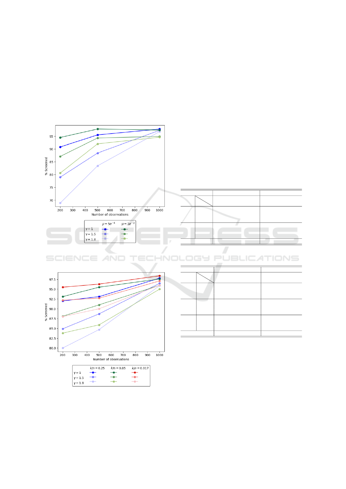
Figure 1: Percentage of features screened as a function of
the number of observations in the dataset and regularization
strength for (REG).
Figure 2: Percentage of features screened as a function of
the number of observations in the dataset and regularization
strength for (CARD).
Figures 1 and 2 show the percentage of fea-
tures eliminated from the regression by the screen-
ing procedure for different regularization strengths for
(REG) and (CARD), respectively. As the number of
observations increases, the number of screened fea-
tures increases as well. We observe the same trend as
the strength of the regularization increases, i.e., higher
values of µ and lower values of γ lead to better screen-
ing. The reason for improved screening with larger
number of observations and stronger regularization
can be explained by the smaller integrity gap of the
conic relaxations, as shown in Tables 1 and 2. Inte-
grality gap of a relaxation is the relative gap between
the optimal objective value of the mixed-integer prob-
lem and the relaxation. Smaller integrality gaps lead
to the satisfaction of a higher number of screening
rules in Propositions 1 and 2.
Table 1: Integrality gap of big-M and conic formulations for
(REG).
Big-M relaxation Conic relaxation
µ
m
γ
1 1.5 1.8 1 1.5 1.8
5e
−4
200 12.91 15.06 16.05 0.01 0.02 0.04
500 8.43 10.18 10.97 7e
−3
0.02 0.03
1,000 6.00 7.15 7.69 7e
−3
9e
−3
0.01
1e
−3
200 15.81 18.94 20.34 0.02 0.04 0.06
500 9.88 12.38 13.51 0.01 0.03 0.04
1,000 7.39 9.23 10.01 0.01 0.03 0.03
Average 10.07 12.16 13.10 0.01 0.03 0.04
Table 2: Integrality gap of big-M and conic formulations for
(CARD).
Big-M relaxation Conic relaxation
k/n
m
γ
1 1.5 1.8 1 1.5 1.8
0.250
200 10.23 13.32 14.86 0.02 0.05 0.07
500 5.27 7.12 8.08 0.01 0.03 0.04
1,000 2.87 3.91 4.46 4e
−3
0.01 0.02
0.050
200 19.49 24.33 26.61 0.03 0.07 0.10
500 10.48 13.82 15.51 0.01 0.03 0.05
1,000 6.14 8.25 9.33 6e
−3
0.02 0.02
0.017
200 41.74 47.70 50.19 0.05 0.10 0.11
500 26.58 32.73 - 0.02 0.06 -
1,000 16.67 21.47 23.78 0.01 0.03 0.04
Average 15.50 19.18 19.10 0.02 0.04 0.06
In Tables 1 and 2, we also compare the strength
of the conic formulation with the big-M formula-
tion. Observe that the integrality gaps produced by the
conic relaxation are very small, on average 0.03% for
the regularized model and 0.04% for the cardinality-
constrained model. On the other hand, the big-M for-
mulation has a much weaker gap, 12% and 18% for
the regularized and constrained models, respectively.
The tighter gaps with the conic formulation signifi-
cantly help speed up the solution time of the branch-
and-bound algorithm, as well as lead to the elimina-
tion of more variables with the screening rules, further
Safe Screening for Logistic Regression with – Regularization
123

Table 3: Solution times for the regularized logistic regression (REG) with and without screening rules.
Time (sec.)
Speed-up
BnB BnB + Screening
µ
m
γ
1 1.5 1.8 1 1.5 1.8 1 1.5 1.8
5e
−4
200 16 136 264 5 58 127 2.9 2.4 2.1
500 25 69 174 6 19 57 4.3 3.7 3.2
1,000 30 35 49 5 6 9 5.3 5.7 5.5
1e
−3
200 10 31 69 3 10 25 3.4 3.0 2.9
500 9 29 38 2 6 8 4.2 4.7 4.8
1,000 39 66 71 6 9 10 6.3 7.1 6.7
Average 21 61 111 5 18 39 4.4 4.4 4.2
Table 4: Solution times for the cardinality-constrained logistic regression (CARD) with and without screening rules.
Time (sec.)
Speed-up
BnB BnB + Screening
k/n
m
γ
1 1.5 1.8 1 1.5 1.8 1 1.5 1.8
0.250
200 16 40 69 4 11 20 4.2 3.6 3.5
500 41 110 256 7 23 68 5.8 4.9 4.2
1,000 30 47 52 4 7 7 6.7 7.0 7.1
0.050
200 73 200 410 12 38 92 6.2 5.5 4.6
500 102 407 1,056 13 61 234 8.1 6.8 5.3
1,000 159 242 287 14 23 28 10.8 10.3 10.0
0.017
200 912 2,267 1,457 92 1,313 1,703 10.2 8.0 6.4
500 1,267 3,548 - 167 1,144 1,971 12.6 9.3 -
1,000 1,166 1,806 2,327 57 153 368 19.9 15.3 14.4
Average 418 963 740 41 308 499 9.4 7.9 6.9
speeding up the optimization.
In order to see the impact of screening procedure
on the overall solution times, we solve the logistic re-
gression problem using the branch-and-bound algo-
rithm with and without screening, and compare the
solution times and speed-up due to screening vari-
ables. The branch-and-bound algorithm for solving
the big-M formulation exceeds our time limit of 12
hours for the larger instances; therefore, we report re-
sults for the perspective formulation only. These re-
sults are shown in Tables 3 and 4. The computation
time for the screening procedure is included when re-
porting the solution times for branch-and-bound with
screening. The reported times are rounded to the near-
est second. On average, we observe a 4.3× and 8.1×
speed-up in computations due to the proposed screen-
ing procedure for (REG) and (CARD), respectively.
The improvement in solution times increases with the
number of observations. Again, a trend of increased
speed-up as the strength of regularization penalty in-
creases is seen, since more features are eliminated a
priori.
4.3 Results on Real Data
In order to test the effectiveness of the proposed
screening procedures on real data, we solve problems
from the UCI Machine Learning Repository (Dua
et al., 2017) (arcene and newsgroups) and genomic
data from the Gene Expression Omnibus Database
(Edgar et al., 2002) (genomic). In particular we focus
on these larger instances of the repository with a high
ratio of features to observations for which regulariza-
tion is more important to avoid overfitting. We solve
these instances using the regularized logistic regres-
sion model (REG), varying the strength of the regu-
larization. As before, a time limit of 12 hours is set
for each run.
The results are summarized in Table 5. For each
instance, at least 92% of the features are screened, and
particularly for the genomic dataset, 99.9% of the fea-
tures are screened for each parameter setting. Over all
instances, on average, 98% of the features are elimi-
nated by the screening procedure before the branch-
and-bound algorithm. Seven out of the 18 runs did not
complete in 12 hours without screening. On the other
hand, with screening, all but one run is completed
within the time limit and always much faster. For
the instances where branch-and-bound with and with-
out screening both terminate within the time limit,
screening leads to on average 13.8× speed-up, with
larger speed-up (up to 25.6×) for the more diffi-
cult instances. For instances where only the branch-
and0bound does not terminate, there is an average of
KDIR 2022 - 14th International Conference on Knowledge Discovery and Information Retrieval
124

Table 5: Results for screening on real datasets using regularized logistic regression (REG).
Time (sec.)
Speed-up
µ γ % Screened BnB BnB + Screening
genomic
n = 22,883
m = 107
5e
−4
0.5 99.9 104 19 5.5
1 99.9 182 17 11.0
1.5 99.9 184 33 5.5
1e
−3
0.5 99.9 152 14 11.0
1 99.9 445 32 13.8
1.5 99.9 384 54 7.1
arcene
n = 10,000
m = 100
5e
−4
0.5 97 25,963 1,013 25.6
1 97 6,999 336 20.8
1.5 92 >12hr 10,925 >4.0
1e
−3
0.5 99 477 32 14.8
1 96 10,044 467 21.5
1.5 95 22,466 1,425 15.7
newsgroups
n = 28,467
m = 1,977
5e
−4
0.5 99.9 >12hr 1,135 >38.1
0.7 99.9 >12hr 8,701 >5.0
1 99 >12hr >12hr n.a
1e
−3
0.5 99.9 >12hr 401 >107.7
0.7 99.9 >12hr 522 >82.8
1 99.7 >12hr 7,439 >5.8
at least 40.5× speed-up. These experimental results
clearly indicate that the proposed screening rules are
very effective in pruning a large number of features
and result in substantial savings in computational ef-
fort for the real datasets as well.
5 CONCLUSION
In this work, we present safe screening rules for
ℓ
0
− ℓ
2
regularized and cardinality-constrained logis-
tic regression. Our numerical experiments show that
a large percentage of features can be eliminated ef-
ficiently and safely via this preprocessing step before
employing branch-and-bound algorithms, particularly
when regularization is strong, leading to significant
computational speed-up. The strength of the conic re-
laxations contribute significantly to the effectiveness
of the screening rules in pruning a large number of
features. We show the conic formulation provides
much smaller integrality gaps compared to the big-M
formulation, making it more suitable for solving ℓ
0
–
ℓ
2
-regularized logistic regression with a branch-and-
bound algorithm and also for the derived screening
rules.
REFERENCES
Akt
¨
urk, M. S., Atamt
¨
urk, A., and G
¨
urel, S. (2009). A strong
conic quadratic reformulation for machine-job assign-
ment with controllable processing times. Operations
Research Letters, 37:187–191.
Atamt
¨
urk, A. and G
´
omez, A. (2019). Rank-one con-
vexification for sparse regression. arXiv preprint
arXiv:1901.10334.
Atamt
¨
urk, A. and G
´
omez, A. (2020). Safe screening rules
for ℓ
0
-regression from perspective relaxations. In In-
ternational Conference on Machine Learning, pages
421–430. PMLR.
Atamt
¨
urk, A., G
´
omez, A., and Han, S. (2021). Sparse
and smooth signal estimation: Convexification of ℓ
0
-
formulations. Journal of Machine Learning Research,
22(52):1–43.
Bertsimas, D., King, A., Mazumder, R., et al. (2016). Best
subset selection via a modern optimization lens. The
Annals of Statistics, 44:813–852.
Bertsimas, D. and Van Parys, B. (2017). Sparse
high-dimensional regression: Exact scalable al-
gorithms and phase transitions. arXiv preprint
arXiv:1709.10029.
Cawley, G. C. and Talbot, N. L. (2006). Gene selection
in cancer classification using sparse logistic regres-
sion with bayesian regularization. Bioinformatics,
22(19):2348–2355.
Dantas, C., Soubies, E., and F
´
evotte, C. (2021). Expand-
ing boundaries of gap safe screening. arXiv preprint
arXiv:2102.10846.
Dedieu, A., Hazimeh, H., and Mazumder, R. (2021). Learn-
ing sparse classifiers: Continuous and mixed integer
optimization perspectives. Journal of Machine Learn-
ing Research, 22(135):1–47.
Dua, D., Graff, C., et al. (2017). UCI machine learning
repository.
Edgar, R., Domrachev, M., and Lash, A. E. (2002). Gene
expression omnibus: Ncbi gene expression and hy-
bridization array data repository. Nucleic acids re-
search, 30(1):207–210.
El Ghaoui, L., Viallon, V., and Rabbani, T. (2010). Safe
Safe Screening for Logistic Regression with – Regularization
125

feature elimination for the lasso and sparse supervised
learning problems. arXiv preprint arXiv:1009.4219.
Fercoq, O., Gramfort, A., and Salmon, J. (2015). Mind
the duality gap: safer rules for the lasso. In Interna-
tional Conference on Machine Learning, pages 333–
342. PMLR.
Gramfort, A., Strohmeier, D., Haueisen, J., H
¨
am
¨
al
¨
ainen,
M. S., and Kowalski, M. (2013). Time-frequency
mixed-norm estimates: Sparse m/eeg imaging with
non-stationary source activations. NeuroImage,
70:410–422.
Han, S., G
´
omez, A., and Atamt
¨
urk, A. (2020). 2x2-
convexifications for convex quadratic optimiza-
tion with indicator variables. arXiv preprint
arXiv:2004.07448.
Hazimeh, H. and Mazumder, R. (2020). Fast best subset
selection: Coordinate descent and local combinato-
rial optimization algorithms. Operations Research,
68(5):1517–1537.
Hoerl, A. E. and Kennard, R. W. (1970). Ridge regression:
Biased estimation for nonorthogonal problems. Tech-
nometrics, 12:55–67.
Kuswanto, H., Asfihani, A., Sarumaha, Y., and Ohwada, H.
(2015). Logistic regression ensemble for predicting
customer defection with very large sample size. Pro-
cedia Computer Science, 72:86–93.
Liu, J., Zhao, Z., Wang, J., and Ye, J. (2014). Safe screen-
ing with variational inequalities and its application to
lasso. In International Conference on Machine Learn-
ing, pages 289–297. PMLR.
Miller, A. (2002). Subset Selection in Regression. CRC
Press.
MOSEK ApS, . (2021). MOSEK Optimizer API for Python.
Release 9.3.13.
Ndiaye, E., Fercoq, O., Gramfort, A., and Salmon, J.
(2017). Gap safe screening rules for sparsity enforcing
penalties. The Journal of Machine Learning Research,
18(1):4671–4703.
Shevade, S. K. and Keerthi, S. S. (2003). A simple and effi-
cient algorithm for gene selection using sparse logistic
regression. Bioinformatics, 19(17):2246–2253.
Tibshirani, R. (1996). Regression shrinkage and selection
via the Lasso. Journal of the Royal Statistical Society.
Series B (Methodological), pages 267–288.
Tibshirani, R. (2011). Regression shrinkage and selection
via the lasso: A retrospective. Journal of the Royal
Statistical Society: Series B (Statistical Methodol-
ogy), 73:273–282.
Wang, J. and Park, E. (2017). Active learning for penalized
logistic regression via sequential experimental design.
Neurocomputing, 222:183–190.
Wang, J., Zhou, J., Liu, J., Wonka, P., and Ye, J. (2014).
A safe screening rule for sparse logistic regression.
Advances in Neural Information Processing Systems,
27:1053–1061.
Wang, J., Zhou, J., Wonka, P., and Ye, J. (2013). Lasso
screening rules via dual polytope projection. In Ad-
vances in Neural Information Processing Systems,
pages 1070–1078. Citeseer.
Yen, S.-J., Lee, Y.-S., Ying, J.-C., and Wu, Y.-C. (2011). A
logistic regression-based smoothing method for chi-
nese text categorization. Expert Systems with Appli-
cations, 38(9):11581–11590.
Zou, H. and Hastie, T. (2005). Regularization and variable
selection via the elastic net. Journal of the Royal Sta-
tistical Society: Series B (Statistical Methodology),
67:301–320.
KDIR 2022 - 14th International Conference on Knowledge Discovery and Information Retrieval
126
