Mathematical Modelling of One-dimensional Fluid Flows Bounded by

a Free Surface and an Impenetrable Bottom

S. L. Deryabin

and A. V. Mezentsev

Ural State University of Railway Transport, Yekaterinburg, Russia

Keywords: One-dimensional fluid flows, free surface, impenetrable bottom, shoreline, breakup of discontinuity, shallow

water equation, non-stationary self-similar variable, analytical solution, convergent series.

Abstract: The paper investigates a one-dimensional model of a wave coming ashore with a subsequent collapse. For

modelling, a system of shallow water equations is taken, which considers the effect of gravity. A non-

stationary self-similar variable is introduced in the system of shallow water equations. For a system of

equations written in new variables, a boundary condition on the sound characteristic is formulated. The power

series is used to construct the solution. Algebraic and ordinary differential equations are solved to find the

coefficients of the series. The convergence of this series is proved. The locally analytical solution of the

problem of wave overturning in the space of physical variables is constructed. The obtained analytical

solutions can be useful for setting boundary and initial conditions in numerical simulation of a tsunami wave

over a long period of time.

1 INTRODUCTION

Approximate shallow water equations are often used

in numerical modelling of tsunami waves coming

ashore. In such models, problems with a movable

boundary are solved, in which the shoreline (the

water-land boundary) moves to the shore. Since the

water depth becomes zero at the shoreline, a feature

appears in the system of equations (Vol’cinger,

Klevannyj, Pelinovskij, 1989). To correctly account

for this feature in calculations, it is necessary to

construct an analytical solution in the vicinity of the

shoreline (Hibberd, Peregrine, 1979). Earlier in

(Carrier, Greenspan, 1958), analytical solutions of a

system of one-dimensional shallow water equations

were obtained to describe the output to a flat slope of

non-collapsing standing waves. In (Carrier, Wu, Yen,

2003) and (Kanoglu, 2004), the dependence of the

trajectory of the point of shoreline on the initial

waveform was considered. The formula for

calculating the maximum value of the wave height on

a flat angular slope was obtained in (Sanolakis, 1987).

The models obtained in (Carrier, Greenspan, 1958;

Carrier, Wu, Yen, 2003; Kanoglu, 2004; Sanolakis,

1987) are approximate, since the coastal slope in them

https://orcid.org/0000-0003-3730-0966

https://orcid.org/0000-0002-5678-8701

is a flat slope, and not a curved surface as it is

observed in nature. The movement of the wave on

such a surface has a more complex form. The main

difficulty here is to model the motion along the

curved surface of the water-land boundary for

crashing waves. This work is devoted to solving this

problem.

Note that the first approximation of the system of

shallow water equations exactly coincides with the

equations of motion of a polytropic gas with the

polytropic exponent γ = 2. In this case, the shoreline

for shallow water equations in the system of gas

dynamics equations is the gas-vacuum boundary. In

(Bautin, Deryabin, 2005), solutions of one-

dimensional and multidimensional problems of

modelling gas motion in vacuum are given. In

(Bautin, Deryabin, 2005) the problem of the breakup

of a special discontinuity is solved. Here is the

formulation of this problem.

It is assumed that the surface Γ separates the gas

from the vacuum. If the density of the gas on one side

of the impenetrable surface of the gas is strictly

greater than zero, and on the other is equal to zero,

then they say that this is the problem of the breakup

of a special discontinuity. In the problem, it is

266

Deryabin, S. and Mezentsev, A.

Mathematical Modelling of One-dimensional Fluid Flows Bounded by a Free Surface and an Impenetrable Bottom.

DOI: 10.5220/0011582800003527

In Proceedings of the 1st International Scientiﬁc and Practical Conference on Transport: Logistics, Construction, Maintenance, Management (TLC2M 2022), pages 266-271

ISBN: 978-989-758-606-4

 2023 by SCITEPRESS – Science and Technology Publications, Lda. Under CC license (CC BY-NC-ND 4.0)

required to describe the movement of gas after the

instant destruction of the wall Γ. The self-similar

solution of such a problem in the one-dimensional

case was first found by B. Riemann for plane-

symmetric flows. In the future, the solution of this

problem was constructed in special functional spaces

after replacing the dependent and independent

variables. Such a solution method became possible in

(Bautin et al., 2011) to describe the overturning of the

wave. The constructed solution has the form of a

power series converging in the vicinity of the

boundary. Using spatial variables, the law of motion

of the water-land boundary is obtained and the values

of the velocity of the liquid on it are found. In this

paper, locally converging series are also constructed

– the solution of the wave overturning problem, but

unlike (Bautin et al., 2011), the solution is constructed

using non-stationary self-similar variables in physical

space.

2 MATERIALS AND METHODS

The characteristic Cauchy problem is taken as the

object of research. In (Bautin, 2009), one can find

formulations and proofs of theorems about the

existence and uniqueness of solutions to such

problems. The method of constructing solutions is as

follows. A nonlinear system of differential equations

describing the physical conservation laws is chosen.

Boundary and initial conditions are set for it using

analytical functions. A local theorem on the existence

and uniqueness of the solution of the initial boundary

value problem is proved. The analytical solution is

constructed in the form of a power series, and its

convergence is proved.

2.1 Statement of the Problem

The flow of an incompressible inviscid fluid without

vortices under the action of gravity is considered. Let

the layer of such a liquid be bounded by a free surface

and an impermeable bottom. The Cartesian

coordinate system is introduced so that the line z = 0

corresponds to the level of the stationary liquid. The

bottom is given by the function z = – h(x).

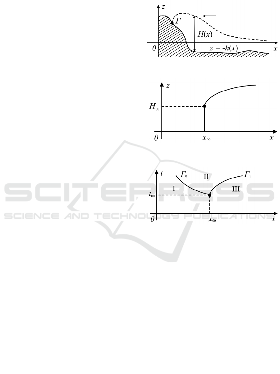
At time t = 0, the liquid wave is separated from

the land by the point Γ (the shoreline). Moreover,

there is a dry shore to the left of Γ, and the sea to the

right (fig. 1).

Figure 1: Wave, shore and shoreline (point) Г.

Figure 2: Waveform at time t = 0.

Figure 3: I — dry shore, II — disturbed wave, III —

undisturbed wave.

Consider the system of shallow water equations in

the first approximation (Ovsyannikov, 2003;

Khakimzyanov et al., 2001):

txx

tx x x

Н uH Hu

uuu gH gh

++=

++ =

(1.1

)

where g is the acceleration of gravity, and the

unknown functions: H is the height of the liquid

measured from the bottom to the upper level of the

liquid, u is the velocity of the liquid. It is also assumed

that at time t = 0 the waveform has the form of a step

with a straight vertical part (fig. 2). The vertical

equation has the form x = x

, and the height of the

vertical part is equal to H

= H

). At the initial

moment of time, the analytical functions are known:

0000

(), (), .uux H Hx xx==>

Mathematical Modelling of One-dimensional Fluid Flows Bounded by a Free Surface and an Impenetrable Bottom

267

Moreover, it is assumed that u(x

) = u

< 0 and for

all x ≥ x

, the values of the function H

(x) > 0 are

strictly positive. The fluid flow defined by such

functions is called the background flow (undisturbed

wave). After overturning the step at time t = 0, a

disturbed wave is formed, which, at t > 0, is separated

from the undisturbed wave by the line Γ

(the line of

weak discontinuity), from the land by the boundary

— the shoreline (the water-land boundary) (fig. 3):

(, )| 0.

Htx =

In the problem, it is required to construct

analytical functions describing the motion of a fluid

in the region of disturbed and undisturbed waves and

the motion of the boundary Γ

. Note that the system

(1.1) and the initial data satisfy the conditions of

Kovalevskaya's theorem. According to this theorem,

its only solution has the form (Bautin, 2009):

(, ), (, ).u u tx H H tx==

In system (1.1), we introduce a new unknown

function:

1/ 2 2

(, ) (, ), ( ).Ctx H tx H C==

After the transformations, we get:

tx x

tx x x

CuC Cu

uuu gCC gh

++ =

(1.2

)

In these new designations, the background flow

will have the form:

00 00

(, ),

(, ) (, ), .

uutx

CCtx HtxC H

== =

Let's write down the differential equation and the

initial condition for the motion of Γ

: x = x

(t)

(Ovsyannikov, 2003):

11 1

(, ) (, ),

utx gCtx=+

100

(0) .

(1.3

)

Problem (1.3) satisfies the conditions of

Kovalevskaya's theorem. According to this theorem,

its solution can be represented as:

() .

xt x

∞



(1.4)

Let's find the coefficients of the series (1.4). The

zero and first coefficients of the series are from (1.3):

10 00 11 00 00

xxu gC==+

The following coefficients of the series are found

by successive differentiation of equation (1.3):

tt t t

ugC=+

Then we get

12 00 00

(0, ) (0, ).

ux gCx=+

According to the obtained formulas, as well as in

(Bautin, 2009), the law of motion x

(t) is written using

the analytical function x

(t) Γ

1002

() ().

xt x txt==+

The boundary conditions on Γ

are given by the

equations:

() 1

( , ) | ( , ( )),

xxt

utx u tx t

() 1

( , ) | ( , ( )).

xxt

Ctx C tx t

(1.5)

To construct a disturbed wave in the system (1.2),

we introduce non-stationary self-similar variables

according to the following formulas:

tty

−

′

The stroke sign is not used in the future.

After the transformations, we get the system:

() 0,

tyy

tC u y C Cu+− + =

()2 ( ),

tyyx

tu u y u gCC tgh x ty+− + = +

(1.6)

with conditions on the characteristic Γ

() 1

(, )| (, ()),

yx t

ut y u tx t

() 1

( , ) | ( , ( )).

yx t

Ct y C tx t

(1.7)

2.2 Construction of a Solution in

Physical Space

To construct a solution of the problem (1.6), (1.7), we

write the power series (Bautin, Deryabin, 2005):

TLC2M 2022 - INTERNATIONAL SCIENTIFIC AND PRACTICAL CONFERENCE TLC2M TRANSPORT: LOGISTICS,

CONSTRUCTION, MAINTENANCE, MANAGEMENT

268

(, ) ( ) , { , }.

ty y uC

∞



fff

(2.1)

We will find the zero coefficients of the series

from the system (1.6) at the value t = 0:

00 00

() 0,

()2 0.

uyC Cu

uyu gCC

−+ =

(2.2)

For the existence of a non-zero solution of the

resulting system (2.2), it is necessary that its

determinant is equal to zero, i.e.

000 0

() , .uy gCuy gC−= −=±

Since at t = 0 on characteristic Γ

we have

(Ovsyannikov, 2003):

00 00

.yu gC=+

Hence, we have:

.uy gC−=−

(2.3)

Substituting u

– y into the second equation of the

system (2.2.), we get:

0000

2,2 ,

ugCugCD==+

where D is determined from the conditions (1.7):

000000

22.ugCu gC=+−

Substituting u

into (2.3.), we get:

00000

(2),

22 1

33 3

CyugC

uygCu

=−+

=− +

(2.4)

The following relations are also valid

Cuy

(2.5)

After differentiating (2.2) at t = 0, considering (2.4),

(2.5), we obtain:

01 0 1 1 1

01 0 1 1 1 10

20,

Cu gCC u C

Cu gCC u C D

−++=

−+ + +=

(2.6)

where

10 00

().

gh x=

When adding the equations of the system (2.6), we

obtain:

11 00

710

()

uCghx

1100

10 3

(),

ugCghx=− +

ugC=−

Substituting u

and u

into the second equation (2.6),

after the transformations we have

01 1 00

().

212

CC C gh x−=

Substituting C

in this equation, after the

transformations we get:

00 00 1 1 00

(2) ().

yu gC C C ghx−+ − =

Integrating the equation, we have:

()

110 00 00

1100000

CCyu gC

ugCyugC

=−+ −

=− − + −

(2.7)

The integration constant C

is determined from the

conditions (1.7). The following coefficients of the

series (2.1) are found from (1.6) by differentiating k

times. After that, we assume t = 0 (Bautin, Deryabin,

2005). So, given (2.3), (2.4), we get:

00 1

00 2

32 2

ky ky k k

ky ky k k k

Cu g CC C F

Cu g CC u C F

−++=

−+ + +=

(2.8)

where the functions F

= F

(y), F

= F

(y) are

determined recursively based on the previously found

coefficients of the series. Adding the first and second

equations of the system (2.8), we get:

14 4

2(),

kkk

ku kCFy

 

+++ =

 

 

Mathematical Modelling of One-dimensional Fluid Flows Bounded by a Free Surface and an Impenetrable Bottom

269

оr

64 3

(),

34 34

kkk

ugCgFy

=− +

64 3

(),

34 34

ky ky ky

ugCgFy

=− +

where

() () ().

kkk

yFy Fy

Substituting u

and u

into the second equation (2.8),

after the transformations we have:

12 12 2 (3 2)

34 3 34

ky k k

CC C F



+− =





Here the function F

= F

(y) has the form:

34 34

kk ky k

FCFF

=+ −

Substituting C

into the equation, after the

transformations we get:

()

00 00 1

334

2().

244

ky k k

yu gC C kC Fy

−+ − =

Integrating this equation, we have:

()

102

102 3

kkk k

kkkkk

CGC G

ugGCGG

=− + +

(2.9)

where

()

20000

() 2 ,

GFyyugCdy

−−

=−+



()

100003

3()

2, .

Gyu gC G

=− + =

The integration constants C

are found from

(1.7). Substitute C = C

(t, x

(t)), y = x

(t) in series

(2.1). As a result, we have

(, ()) (, ()).Ctx t C tx t=

Differentiating this relation and substituting t = 0,

we get the equations for finding the coefficients:

()

0000

:3 .

kkk

CgCCQ=

Here the function Q

is a known constant. Since

≠ 0, then C

are uniquely determined. Thus, the

uniqueness of the formal solution of the problem

(1.6), (1.7) constructed in the form of a series (2.1) is

proved.

Theorem 1. Problem (1.6), (1.7) has a unique

analytical solution, which is the convergent series

(2.1).

The proof of the theorem is carried out by the

majorant method, the application of which to the

characteristic Cauchy problem is described in detail

in (Bautin, 2009) and is not given in this paper. Using

the simplest transformations, the solution (2.1) is

written in the physical space of variables t, x:

00 00

,,,.

xx xx

HCt uut

−−







3 RESULTS AND DISCUSSION

Previously, the problem of the breakup of a special

discontinuity were solved (Bautin, Deryabin, 2005;

Bautin et al., 2011) in the space of specially

introduced new independent variables. At the same

time, in the space of the initial physical variables, the

laws of motion of the surfaces Γ

, Γ

were determined

explicitly. But in order to determine the values of gas-

dynamic parameters in the space of physical variables

at some point in time t = t

, it was necessary to reverse

the implicitly specified functions. This procedure is

rather cumbersome and difficult for setting the initial

data at time t = t

> 0 between the surfaces Γ

and Γ

for the subsequent construction of the gas flow by

numerical methods. To overcome the difficulty of

inverting implicitly given functions this article solves

the problem of wave overturning by introducing non-

stationary self-similar variables. In this case, the gas

parameters at time t = t

> 0 are determined explicitly

in the space of the initial physical independent

variables using the initial segments of the converging

series (2.1).

Note that the constructed solution (2.1) allows us

to obtain an approximation of the initial conditions at

time t = t

in the form of the initial segments of the

series. Also, the formulas (1.4), (1.5) give an

approximation of the boundary conditions on the line

4 CONCLUSIONS

In this paper, the locally analytical solution of the

problem of wave overturning in the space of physical

variables is constructed. In the form of a convergent

TLC2M 2022 - INTERNATIONAL SCIENTIFIC AND PRACTICAL CONFERENCE TLC2M TRANSPORT: LOGISTICS,

CONSTRUCTION, MAINTENANCE, MANAGEMENT

270

series, the initial conditions at time t = t

are obtained.

In the form of a converging series, the boundary

conditions are obtained on the boundary of an

undisturbed and disturbed wave.

Thus, the analytical study was carried out for

numerical simulation of the flow that arose after the

collapse of the wave for a long period of time

(Khakimzyanov et al., 2001; Bautin et al., 2011).

REFERENCES

Vol’cinger, N. E., Klevannyj, K. A., Pelinovskij, E. N.,

1989. Long-wave dynamics of the coastal zone,

Gidrometeoizdat. Leningrad, p. 272.

Hibberd, S., Peregrine, D., H., 1979. Surf and run-up on a

beach: a uniform bore. Journal of Fluid Mechanics. 95

(2), pp. 323–345.

Carrier, G. F., Greenspan, H. P., 1958. Water waves of

finite amplitude on a sloping beach. Journal of Fluid

Mechanics. 4 (1). pp. 97–109.

Carrier, G. F., Wu, T. T., Yen, H., 2003. Tsunami run-up

and draw-down on a plane beach. Journal of Fluid

Mechanics. 475. pp. 79–99.

Kanoglu, U., 2004. Nonlinear evolution and runup–

rundown of long waves over a sloping beach. Journal

of Fluid Mechanics. 513. pp. 363–372.

Sanolakis, C. E., 1987. The runup of solitary waves.

Journal of Fluid Mechanics. 185. pp. 523–545.

Bautin, S. P., Deryabin, S. L., 2005. Mathematical

modeling of ideal gas outflow into vacuum, Science.

Novosibirsk, p. 390.

Bautin, S. P., Deryabin, S. L., Sommer, A. F.,

Khakimzyanov, G. S., Shokina, N. Yu., 2011. Use of

analytic solutions in the statement of difference

boundary conditions on movable shoreline. Russian

Journal of Numerical Analysis and Mathematical

Modeling. 26 (4). pp. 353-377.

Bautin, S. P., 2009. The characteristic Cauchy problem and

its applications in gas dynamics, Science. Novosibirsk,

p. 368.

Ovsyannikov, L. V., 2003. Lectures on the fundamentals of

gas dynamics, Institute of Computer Research.

Moscow, Izhevsk. p. 336.

Khakimzyanov, G. S., Shokin, Yu. I., Barahnin, V. B.,

Shokina, N. Yu., 2001. Numerical simulation of fluid

flows with surface waves, SB RAS. Novosibirsk. p. 394.

Mathematical Modelling of One-dimensional Fluid Flows Bounded by a Free Surface and an Impenetrable Bottom

271