
An Improved Method for Determining the Pressure on the Surface of
Backfill Bridges
Anatoly Sergeevich Permikin
1,2 a
, Konstantin Yurievich Astankov
1,2
, Ilya Alexandrovich Osokin
1
,
Nikita Vyacheslavovich Volkov
2
and Igor Georgievich Ovchinnikov
1
1
Ural State University of Railway Transport, Yekaterinburg, Russia
2
Mascot LLC, Yekaterinburg, Russia
Keywords: The backfill bridge, the Boussinesq problem, distribution of stresses in the ground, determination of
displacements, the theory of a linearly deformable half-space.
Abstract: The article discusses the application of the solution of the Boussinesq problem to determine the pressure on
the load-bearing arched structure element of a soil-filled bridge structure, taking into account: the distribution
of pressure in the soil from the test static load along the widths of the roof of the bearing element, the
horizontal component of the pressure from the impact of the static test load, the repulsion of the soil mass due
to the introduction bed rest. As a result, the values obtained in the study of the displacements of sections of
the bearing element at characteristic points with the values obtained during field tests of a road bridge in the
Vologda Region at 156 km of the A—114 Vologda - Novaya Ladoga highway.
1 INTRODUCTION
Currently, the spread of backfill bridges is limited due
to many factors, one of which is the lack of a simple
and logically reflecting the work of the design of the
methodology for taking into account temporary loads
(Heger, 1982; Heger, 1985).
Such artificial structures are calculated using finite
element models created in modern automated software
systems (Rubin, 2016; Shamshina, 2018; Permikin,
2020). However, the results obtained with such
calculations are difficult to analyze and verify, and the
values of the forces in the structural elements are often
overestimated (Safronov, 2010). The models
themselves are difficult to construct and perceive, and
modeling of soil backfill with a lack of experience in
designing soil-filling structures is difficult to
implement due to the unpredictable behavior of the
soil mass over time (Kevin, 2016; Erdogmus, 2010).
In the course of previous research on the topic of
an analytical approach to modeling the distribution of
pressure from a temporary load (Volkov, 2019), it was
noted that the application of the solution of the
Boussinesq problem (Khan, 1988; Gorbunov-
Posadov, 1985) to determine the pressure on the load-
bearing structural element gives unsatisfactory errors
a
https://orcid.org/0000-0002-6162-156X
based on the results of comparing the deflections
obtained with the deflections obtained during static
load tests of the bridge.
The authors propose to improve the laws of
pressure distribution and achieve greater convergence
of the calculation results with the results of full-scale
static tests by introducing the following calculation
provisions:
1. accounting for the distribution of pressure in
the soil thickness from the static test load along the
width of the arch of the bearing element;
2. taking into account the horizontal component
of the pressure from the impact of a static test load;
3. taking into account the resistance of the soil
massif by introducing the coefficient of subgrade
reaction.
To confirm the consistency of the method
proposed by the authors for collecting temporary
loads on the bearing element of a backfill bridge, a
correlation was carried out between the values
obtained during the study of the displacement of the
sections of the bearing element at characteristic points
with the values obtained during field tests of a road
bridge in the Vologda Region at 156 km of the A—
114 Vologda - Novaya Ladoga highway (Safronov,
2010).
Permikin, A., Astankov, K., Osokin, I., Volkov, N. and Ovchinnikov, I.
An Improved Method for Determining the Pressure on the Surface of Backfill Bridges.
DOI: 10.5220/0011584000003527
In Proceedings of the 1st International Scientific and Practical Conference on Transport: Logistics, Construction, Maintenance, Management (TLC2M 2022), pages 291-299
ISBN: 978-989-758-606-4
Copyright
c
2023 by SCITEPRESS – Science and Technology Publications, Lda. Under CC license (CC BY-NC-ND 4.0)
291
2 INITIAL DATA
The physical and mechanical properties of the soil
massif were adopted based on the results of
laboratory studies and field tests that have been
preserved since the construction (Table 1).
Table 1: The physical and mechanical properties of the
soil massif
Modulus of
deformation
E, MPa
Poisson's
ratio v
Coefficient
of
adhesion c,
MPa
Internal
friction
angle
φ,
degrees
Ultimate
tensile
stress R
t
, MPa
22.6 0.3 0.001 30 0
To obtain the displacements of the arch nodes in
characteristic sections, the authors propose to use the
PC "LIRA-CAD".
As initial data, the concentrated loads from the
wheels of a three-axle car Ni, the coordinates of the
points of forces x of the application of loads, the
radius of the arch of the backfill bridge R, the width
of the arch along the ground B were used.
The vertical pressure from the filling ground and
the own weight of the structure are not taken into
account, since during field tests it was the relative
displacements of the sections from the static test load
that were measured.
3 BUILDING A GEOMETRIC
SCHEME
As a design scheme, a two-hinged, once statically
indeterminate circular arch with a radius along the
neutral axis R = 6 m, the width of the arch along the
edge of the filling B = 14 m, the total width of the arch
b = 16 m was adopted. When constructing a
geometric scheme, the curved elements of the arch
between the nodes located on the axis were replaced
by rectilinear rods due to the specifics of constructing
flat calculation schemes in the Lira PC.
The step of the arrangement of nodes with
numbers i = 1,3—49 on the x axis in the geometric
scheme is 0.5 m. Then each of the 24 circular
segments obtained was divided in half by the bisector,
and the intersection points of the bisector and the
neutral axis were modeled by nodes numbered
i=2,4—48. Number of nodes – 49 pcs. Number of
rods -48 pcs.
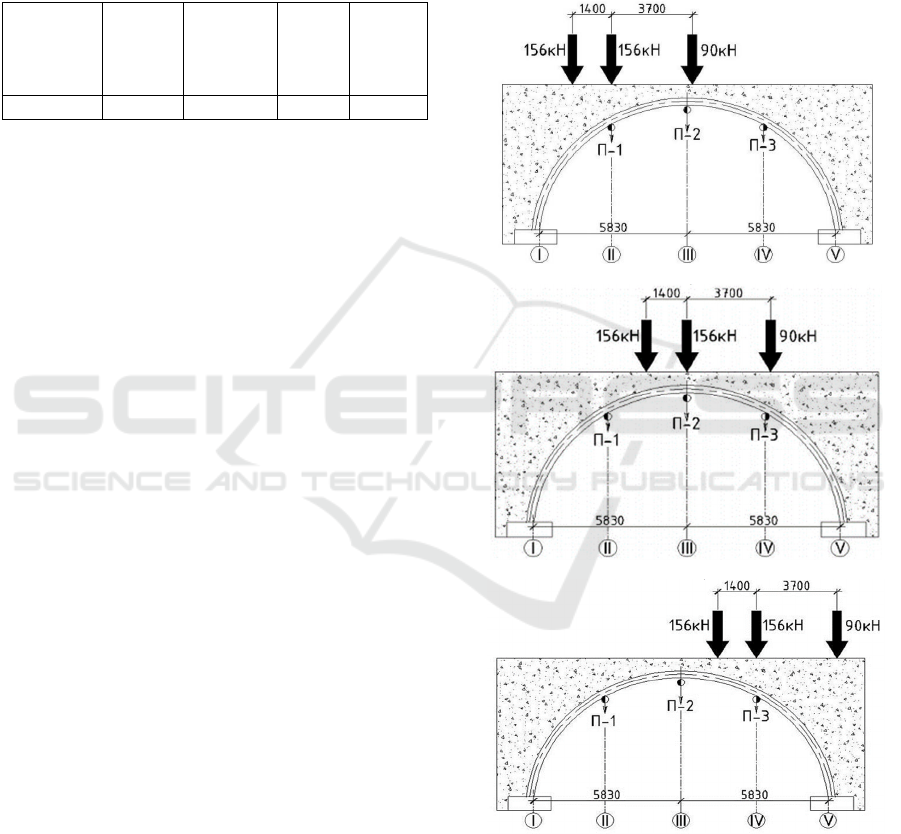
The load from a three-axle VOLVO FM 400 car
with a total weight of 41 tons with a load on the rear
trolley of 312 kN and the front axle of 90 kN will be
taken as six concentrated forces (from each wheel in
three axes) 𝑁
,
=78 кН; 𝑁
,
=78 кН; 𝑁
,
=
45 кНand positioned symmetrically relative to the
axis of the roadway with coordinates𝑦 = ±1,05 м,
and relative to the arch lock - according to the loading
schemes shown in Figures 1, 2, 3. Loading schemes
in Figure 1 correspond to loading schemes when
measuring deflections in sections n=II, III, IV
(Safronov, 2010).
A)
B)
C)
Figure 1: Schemes of loading the bridge with a test load
when measuring deflections in the section a) n = II
(Safronov, 2010); b) n= III (Safronov, 2010); c) n= IV
TLC2M 2022 - INTERNATIONAL SCIENTIFIC AND PRACTICAL CONFERENCE TLC2M TRANSPORT: LOGISTICS,
CONSTRUCTION, MAINTENANCE, MANAGEMENT
292

(
2
)
(
3
)
4 DETERMINATION OF
VERTICAL PRESSURE ON THE
ARCH SURFACE
The law of distribution and transmission of vertical
pressure in a soil massif along the length of the arch
span is generally accepted in the form of the
Boussinesq problem (Khan, 1998):
𝑝
=
∙
∙
∙∙
(
)
,
, (1)
where p
jnz
is the value of the transmitted vertical
pressure from the force N
j
at the point of the half-
space in the section n, kN/m
2
(n=II, III, IV);
N
j
is the value of the concentrated load from the
wheel , kN (j=1, 2, 3, 4, 5, 6);
z is the depth of the point at which the pressure is
determined;
x is the coordinate of the horizontal projection of
the point at which the pressure is determined, relative
to the arch lock.
The laws of vertical pressure change
𝑝
(𝑥,𝑦)have the following form, shown in Figures
2, 3, 4
Figure 2: Stress distribution p
II
z
on the surface of the arch.
Figure 3: Stress distribution p
III
z
on the surface of the arch.
Figure 4: Stress distribution p IV z on the surface of the
arch.
Laws of change of vertical distributed force P
j
II
z
, P
j
III
z
, P
j
IV
z
(kN/m), allowing to determine the load
at any point located on the axis of the arch, from each
of the concentrated forces N
j
have the form.
𝑃
,
(𝑥)
= 117
∙
((
36 – 𝑥
)
.
– 6.67
)
π∙
(((
36 – 𝑥
)
.
–6.67
)
+
(
𝑥+4.4
)
+ (𝑦 ± 1,05)
)
.
𝑑𝑦
𝑃
,
(𝑥)
= 117
∙
((
36 – 𝑥
)
.
– 6.67
)
π∙
(((
36 – 𝑥
)
.
–6.67
)
+(𝑥+3)
+ (𝑦 ± 1,05)
)
.
𝑑𝑦
𝑃
,
(𝑥)
= 67,5
∙
((
36 – 𝑥
)
.
– 6.67
)
π∙
(((
36 –𝑥
)
.
–6.67
)
+
(
𝑥 – 0.7
)
+ (𝑦 ± 1,05)
)
.
𝑑𝑦
𝑃
,
(𝑥)
= 117
∙
((
36 – 𝑥
)
.
– 6.67
)
π∙
(((
36 – 𝑥
)
.
–6.67
)
+
(
𝑥+1.4
)
+ (𝑦 ± 1,05)
)
.
𝑑𝑦
𝑃
,
(𝑥)
= 117 ∙
((
36 – 𝑥
)
.
– 6.67
)
π∙
(((
36 – 𝑥
)
.
–6.67
)
+ 𝑥
+ (𝑦 ± 1,05)
)
.
𝑑𝑦
𝑃
,
(𝑥)
= 67,5
∙
((
36 – 𝑥
)
.
– 6.67
)
π∙
(((
36 –𝑥
)
.
–6.67
)
+
(
𝑥 – 3.7
)
+ (𝑦 ± 1,05)
)
.
𝑑𝑦
(4)
(
5
)
(6)
(7)
An Improved Method for Determining the Pressure on the Surface of Backfill Bridges
293
𝑃
,
(𝑥)
= 234
∙
((
36 – 𝑥
)
.
– 6.67
)
π∙
(((
36 – 𝑥
)
.
– 6.67
)
+
(
𝑥−1.6
)
+ (𝑦 ± 1,05)
)
.
𝑑𝑦
𝑃
,
(𝑥)
= 234
∙
((
36 – 𝑥
)
.
– 6.67
)
π∙
(((
36 – 𝑥
)
.
– 6.67
)
+(𝑥−3)
+ (𝑦 ± 1,05)
)
.
𝑑𝑦
𝑃
,
(𝑥)
= 135
∙
((
36 –𝑥
)
.
– 6.67
)
π∙
(((
36 –𝑥
)
.
– 6.67
)
+
(
𝑥 – 6.7
)
+ (𝑦 ± 1,05)
)
.
𝑑𝑦
The laws of pressure change are compiled taking
into account the minimum filling thickness along the
road axis of 0.67 m (Safronov, 2010).
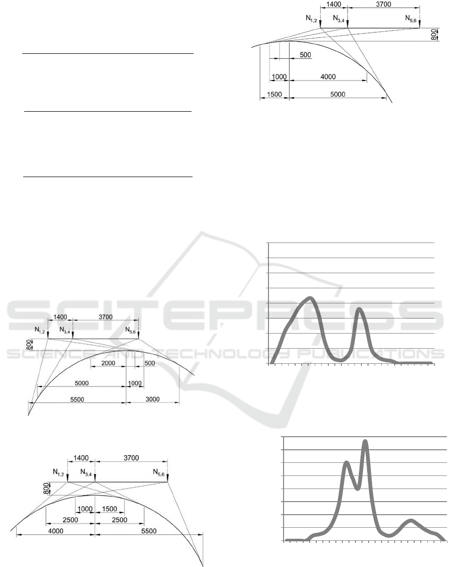
The area of determination of the laws (2) — (10)
along the x axis are the intervals selected taking into
account the possibility of transferring pressure from a
concentrated force. The boundaries of the intervals
are the points of contact with the surface of the arch
of radius vectors originating at the place of
application of loads N
j
(Figures 5, 6, 7).
Figure 5: Places where the radius vectors touch the arch
surface. Section n=II.
Figure 6: Places where the radius vectors touch the arch
surface. Section n=III.
Figure 7: Places where the radius vectors touch the arch
surface. Section n=III.
The total ordinates of pressure P
nz
over the entire
span of the arch for each of the sections n are found
by the superposition principle
𝑃
=
∑
𝑃
. (11)
The laws of load change 𝑃
(𝑥) have the
following form, presented in Figures 8, 9, 10.
Figure 8: Distributed load values P
II
z
along the longitudinal
axis of the arch.
Figure 9: Distributed load values P
III
z
along the
longitudinal axis of the arch.
0
20
40
60
80
100
120
140
160
-6,0
-5,0
-4,0
-3,0
-2,0
-1,0
0,0
1,0
2,0
3,0
4,0
5,0
6,0
Pz, кН/м
x, м
0
20
40
60
80
100
120
140
160
-6,0
-5,0
-4,0
-3,0
-2,0
-1,0
0,0
1,0
2,0
3,0
4,0
5,0
6,0
Pz, кН/м
x, м
(
8
)
(
9
)
(10)
TLC2M 2022 - INTERNATIONAL SCIENTIFIC AND PRACTICAL CONFERENCE TLC2M TRANSPORT: LOGISTICS,
CONSTRUCTION, MAINTENANCE, MANAGEMENT
294

Figure 10: Distributed load values P
IV
z
along the
longitudinal axis of the arch.
5 DETERMINATION OF
HORIZONTAL PRESSURE ON
THE ARCH SURFACE
The law of distribution and transmission of vertical
pressure in a soil massif along the length of the arch
span is generally accepted in the form of the
Boussinesq problem (Khan, 1998):
𝑝
=
∙
∙
∙
∙∙
(
)
,
, (11)
notation in formula (11) – see notation in formula
(1).
The laws of change of horizontal pressure Pjnx
from each of the concentrated forces along the span
length have the form
𝑃
,
(𝑥)
= 117
∙
((
36 – 𝑥
)
.
– 6.67
)
∙(𝑥+4.4)
π∙
(((
36 – 𝑥
)
.
– 6.67
)
+
(
𝑥 + 4.4
)
+ (𝑦 ±1,05)
)
.
𝑑𝑦
(12)
𝑃
,
(𝑥)
= 117
∙
((
36 – 𝑥
)
.
– 6.67
)
∙(𝑥+3.0)
π∙
(((
36 – 𝑥
)
.
– 6.67
)
+ (𝑥+3.0)
+ (𝑦 ±1,05)
)
.
𝑑𝑦
(13)
𝑃
,
(𝑥)
= 67.5
∙
((
36 –x
)
.
– 6.67
)
∙ (𝑥− 0.7)
π∙
(((
36 –x
)
.
– 6.67
)
+
(
x – 0.7
)
+ (y ± 1,05)
)
.
𝑑𝑦
(14)
𝑃
,
(𝑥)
= 117
∙
((
36 – 𝑥
)
.
– 6.67
)
∙(𝑥+1.4)
π∙
(((
36 – 𝑥
)
.
–6.67
)
+
(
𝑥+1.4
)
+ (𝑦 ±1,05)
)
.
𝑑𝑦
(15)
𝑃
,
(𝑥)
= 117 ∙
((
36 – 𝑥
)
.
– 6.67
)
∙𝑥
π∙
(((
36 – 𝑥
)
.
– 6.67
)
+ 𝑥
+ (𝑦 ±1,05)
)
.
𝑑𝑦
(16)
𝑃
,
(𝑥)
= 67.5
∙
((
36 –x
)
.
– 6.67
)
∙ (𝑥− 3.7)
π∙
(((
36 –x
)
.
–6.67
)
+
(
x–3.7
)
+ (y ± 1,05)
)
.
𝑑𝑦
(17)
𝑃
,
(𝑥)
= 117
∙
((
36 – 𝑥
)
.
– 6.67
)
∙(𝑥−1.6)
π∙
(((
36 – 𝑥
)
.
– 6.67
)
+
(
𝑥 − 1.6
)
+ (𝑦 ±1,05)
)
.
𝑑𝑦
(18)
𝑃
,
(𝑥)
= 117
∙
((
36 – 𝑥
)
.
– 6.67
)
∙(𝑥−3.0)
π∙
(((
36 – 𝑥
)
.
– 6.67
)
+ (𝑥−3.0)
+ (𝑦 ±1,05)
)
.
𝑑𝑦
(19)
𝑃
,
(𝑥)
= 67.5
∙
((
36 –x
)
.
– 6.67
)
∙ (𝑥− 6.7)
π∙
(((
36 –x
)
.
– 6.67
)
+
(
x – 6.7
)
+ (y ± 1,05)
)
.
𝑑𝑦
(20)
The area of determination of the laws (12) — (20)
along the x axis are the intervals selected taking into
account the possibility of transferring pressure from a
concentrated force (see Figures 7, 8, 9).
The total pressure ordinates Pnx over the entire
span of the arch for each of the sections n are found
by the superposition principle
𝑃
=𝑃
. (21)
It is worth noting that the rods with node numbers
1-25 are assigned only those loads P
n x
that have a
positive direction relative to the x axis, that is, with a
positive sign before the ordinates. Rods with node
numbers 25-49 are assigned only those loads P
n x
that
have a negative direction relative to the x axis, that is,
with a negative sign before the ordinates.
0
20
40
60
80
100
120
140
160
-6,0
-5,0
-4,0
-3,0
-2,0
-1,0
0,0
1,0
2,0
3,0
4,0
5,0
6,0
Pz, кН/м
x, м
An Improved Method for Determining the Pressure on the Surface of Backfill Bridges
295

Ordinate values of distributed loads P
II
z
, P
III
z
, P
IV
z
, P
II
x
, P
III
x
, P
IV
x
are shown in table 2.
6 DETERMINATION OF
COEFFICIENTS OF
SUBGRADE REACTION
The coefficients of subgrade reaction c
1
for each rod
are calculated in accordance with Appendix B (SP
24.13330.2011 ). The coefficient of subgrade reaction
in the Lira PC acts in the direction of the local axis of
the rod z. The calculated value of the coefficient of
subgrade reaction is found by the formula
𝑐
=𝑐
/𝑠𝑖𝑛ε,
(22)
The coefficient of subgrade reaction is set only to
those rods whose movement occurs "beyond" the
contour of the undeformed circuit.
The values of the coefficients of subgrade
reaction for the left half of the arch are given in Table
3. The values of the coefficients of subgrade reaction
for the right half of the arch are similar to those given.
7 DETERMINATION OF
DISPLACEMENTS
To determine the displacements of the desired
sections z
k
, the authors proposed to use the Mohr
method using the rule of A.K. Vereshchagin (Volkov,
2019; Polyakov, 2011).
The displacements were calculated taking into
account the influence of longitudinal forces and
shearing forces arising in the rods according to the
formulas (Polyakov, 2011 ):
𝑍
=
𝑀
𝑀
𝐸𝐼
𝑑𝑥+
𝑁
𝑁
𝐸𝐴
𝑑𝑥+
𝑄
𝑄
𝐺𝐴
𝑑𝑥,
𝑋
=
𝑀
𝑀
𝐸𝐼
𝑑𝑥+
𝑁
𝑁
𝐸𝐴
𝑑𝑥+
𝑄
𝑄
𝐺𝐴
𝑑𝑥,
Table 2: Ordinate values of distributed loads.
x, m i P II z, kN/m
P III z,
kN/m
P IV z, kN/m P II x, kN/m P III x, kN/m P IV x, kN/m
-6.0 1 - - - - - -
-5.5 3 19.67 - - -5.06 - -
-5.0 5 43.02 - - -14.25 - -
-4.5 7 57.59 - - -13.13 - -
-4.0 9 73.02 7.72 - -6.36 -9.13 -
-3.5 11 82.75 9.79 - 4.42 -11.44 -
-3.0 13 85.90 14.15 - 17.64 -15.36 -
-2.5 15 66.60 27.63 - 35.30 -28.42 -
-2.0 17 28.21 57.78 - 27.81 -39.85 -
-1.5 19 8.98 119.41 0.58 11.85 -25.37 -2.10
-1.0 21 4.36 97.55 0.94 2.05 19.33 -3.51
-0.5 23 5.99 81.72 1.57 -5.59 -19.41 -5.22
0.0 25 19.95 153.44 3.64 -18.46 10.28 -9.42
0.5 27 70.85 64.02 12.23 -19.07 49.43 -21.01
1.0 29 56.79 18.75 51.42 23.34 24.89 -44.84
1.5 31 19.15 8.99 119.45 17.81 11.85 -25.64
2.0 33 8.07 7.95 98.59 10.35 1.54 3.66
2.5 35 4.61 15.03 94.06 6.83 -5.82 -0.30
3.0 37 3.27 25.85 86.60 5.10 -12.28 15.86
3.5 39 - 31.06 61.54 - -3.46 22.97
4.0 41 - 25.03 44.18 - 3.42 19.16
4.5 43 - 17.77 28.74 - 5.26 5.65
5.0 45 - 12.65 26.25 - 4.90 4.00
5.5 47 - 9.25 11.08 - 3.90 -3.11
6.0 49 - - 7.46 - - -0.78
TLC2M 2022 - INTERNATIONAL SCIENTIFIC AND PRACTICAL CONFERENCE TLC2M TRANSPORT: LOGISTICS,
CONSTRUCTION, MAINTENANCE, MANAGEMENT
296

where M
nz
, Q
nz
, N
nz
are diagrams of bending
moments, longitudinal forces and shearing forces
from the action of the test load in sections n;
M
kz
, Q
kz
, N
kz
– diagrams of bending moments,
longitudinal forces and shearing forces from the
action of a single load in the direction of the z axis at
node k;
M
kx
, Q
kx
, N
kx
– diagrams of bending moments,
longitudinal forces and shearing forces from the
action of a single load in the direction of the x axis at
node k;
E – modulus of elasticity of the construction
material;
G is the shear modulus of the construction
material;
I
red
is the axial moment of inertia of the reduced
section;
A
red
is the area of the reduced section.
It is advisable to compare with the results of field
tests the displacements from the Lira PC, calculated
by the formula
Δ
=
𝑋
+𝑍
,
where X
n k
is the horizontal displacement of the k-
th characteristic section of the arch;
Z
n k
— vertical displacement of the k-th
characteristic section of the arch;
Δ
nk
is the total displacement of the k-th
characteristic section of the arch.
Displacements X
n k
and Z
n k
The complete
displacements of the characteristic cross sections of
the arch Δ
n k
, mm, located in 0.25 L, 0.5 L and 0.75 L
span are shown in Table 4.
Table 4: Calculated displacements of characteristic
sections.
k x
k
,m Δ
II k
, mm Δ
III k
, mm
Δ
IV k
,
mm
1 -3 -0.16 -0.13 0.14
2 0 -0.14 -0.36 -0.17
3 3 0.10 -0.12 -0.22
Table 3: Calculation of coefficients of subgrade reaction.
i
The depth of the center
of gravity of the rod, m
Proportionality
coefficient, kN/m
4
Coefficient of subgrade
reaction c
1
, kN/m
3
α
Coefficient of subgrade
reaction c
z
, kN/m
3
24 25 0.67
6,000
4020 0.017 230341
23 24 0.68 4080 0.070 58489
22 23 0.7 4,200 0.105 40180
21 22 0.74 4440 .139 31903
20 21 0.78 4680 0.191 24527
19 20 0.83 4980 0.225 22138
18 19 0.9 5,400 0.276 19591
17 18 0.97 5820 0.309 18834
16 17 1.06 6360 0.358 17747
15 16 1.16 6960 0.342 20350
14 15 1.27 7620 0.485 15718
13 14 1.41 8460 0.485 17450
12 13 1.55 9300 0.515 18057
11 12 1.71 10260 0.559 18348
10 11 1.9 11400 0.602 18943
9 10 2.09 12540 0.643 19509
8 9 2.32 13920 0.695 20039
7 8 2.57 15420 0.731 21084
6 7 2.86 17160 0.777 22081
5 6 3.19 19140 0.805 23780
4 5 3.58 21480 0.865 24821
3 4 4.04 24240 0.904 26819
2 3 4.86 29160 0.951 30655
1 2 6.06 36360 0.992 36658
An Improved Method for Determining the Pressure on the Surface of Backfill Bridges
297

8 COMPARISON OF THE
OBTAINED RESULTS WITH
THE RESULTS OF A
FULL-SCALE EXPERIMENT
For the convenience of comparing the existing results
with the results obtained, we will summarize them in
Table 5.
9 CONCLUSIONS
We hope you find the information in this template
useful in the preparation of your submission.
Comparing the calculated values of Δk with the
calculated values obtained by modeling the structure
in the Lira PC zk, as well as with the displacements
obtained during full-scale tests of ze, it can be noted
that the values calculated according to the method
proposed by the authors have deviations of up to 17
percent from the values obtained during full-scale
tests. It is also worth noting that the deviations of the
results obtained during the study are 5 times less than
the deviations obtained during the calculation in
(Volkov, 2019) when compared with the results of
field tests.
Thus, the computational model using the theory
of a linearly deformable half-space proposed by the
authors for calculating the pressure acting from
temporary loads reliably reflects the work of backfill
structures, which allows us to apply the problems of
elasticity theory with a sufficient degree of accuracy
to describe the distribution of stresses in the soil from
temporary loads when collecting loads on the load-
bearing elements of backfill bridges.
REFERENCES
Safronov, V. S., Zazvonov, V. V., 2010. Full-scale static
tests of a backfill road bridge with a vaulted span
made of monolithic reinforced concrete. Construction
mechanics and structures, No. 1., pp. 29-38.
Volkov, N. V., Permikin, A. S., 2019. Analytical
calculation of a backfill bridge. Perspective, No. 2.,
pp. 4-18.
Khan, H., 1988. Theory of Elasticity: Fundamentals of
linear theory and its application: textbook. Mir, 344 p.
SP 24.13330.2011 with amendments No. 1, 2, 3. Pile
foundations: set of rules: official publication:
approved and put into effect by Order of the Ministry
of Regional Development of the Russian Federation
(Ministry of Regional Development of Russia) dated
December 27, 2010 N 786: updated version of SNiP
2.02.03-85: date of introduction 20-05-2011.
Developed by N.M. Gersevanov Research Institute –
Institute of JSC "Research Center "Construction",
2019.Standartinform.
Polyakov, A. A., Koltsov, V. M., 2011. The resistance of
materials and the fundamentals of the theory of
elasticity: textbook 2nd ed.revised and corrected.
UrFU, 527 p.
Rubin, O. D., Lisichkin, S. E., Shestopalov, P. V., 2016.
Features of mathematical finite element modeling of
systems "concrete structure under construction - non-
rock foundation". In construction mechanics of
engineering structures and buildings. No. 2., pp. 63-
67.
Gorbunov-Posadov, M. I., Ilyichev, V. A., Krutov, V. I.,
1985. Bases, foundations and underground structures:
designer's handbook. Stroyizdat,480 p.
Shamshina, K. V., Migunov, V. N., Ovchinnikov, I. G.,
2018. IOP Conf. Ser.: Mater. Sci. Eng. 451, 012058.
Permikin, A. S., Ovchinnikov, I. G., and Gricuk, A. I.,
2020. Russian Journal of Transport Engineering 4.
Spangler, M. G., 1960. Soil engineering 2nd ed. Scranton:
International textbook company.
Table 5: Comparison of calculation results.
Displacements in calculated sections,
Calculated cross sections, k
1 2 3
measured during field tests z
n e
, mm
z
II e
, mm -0.33 -0.10 0.08
z
III e
, mm -0.12 -0.41 -0.06
z
IV e
, mm 0.10 -0.20 -0.30
calculated in the article (Volkov, 2019) z
n k
,
mm
z
II k
, mm — — —
z
III k
, mm -0.14 -0.78 -0.36
z
IV k
, mm — — —
calculated by the improved method in this
paper Δ
n k
, mm
Δ
II k
, mm -0.16 -0.14 0.10
Δ
III k
, mm -0.13 -0.36 -0.12
Δ
IV k
, mm 0.14 -0.17 -0.22
TLC2M 2022 - INTERNATIONAL SCIENTIFIC AND PRACTICAL CONFERENCE TLC2M TRANSPORT: LOGISTICS,
CONSTRUCTION, MAINTENANCE, MANAGEMENT
298

Heger, F. J., Transportation Research Board 878, 1982.
pp. 93-100.
Heger, F. J., Liepins, A. A., Selig, E. T., 1985.
Transportation Research Board 1008.
Kevin, L. A., 2016. A review of depth of cover tables for
concrete and corrugated metal pipe for the Iowa
Depatment of Transportation.
Erdogmus, E., Skourup, B. N., Tadros, M., 2010. Journal
of pipeline systems and practice 1, pp. 25-32.
An Improved Method for Determining the Pressure on the Surface of Backfill Bridges
299
