
Generalization of Probabilistic Latent Semantic Analysis to k-partite
Graphs
Yohann Salomon
1
and Pietro Pinoli
2
1
ENSTA, Palaiseau, France
2
Department of Electronics, Information and Bioengineering, Politecnico di Milano, Milan, Italy
Keywords:
PLSA, EM-algorithm, k-partite Graphs, Link Prediction.
Abstract:
Many data can be easily modelled as bipartite or k-partite graphs. Among the many computational analyses
that can be run on such graphs, link prediction, i.e., the inference of novel links between nodes, is one of the
most valuable and has many applications on real world data. While for bipartite graphs many methods exist for
this task, only few algorithms are able to perform link prediction on k-partite graphs. The Probabilistic Latent
Semantic Analysis (PLSA) is an algorithm based on latent variables, named topics, designed to perform matrix
factorisation. As such, it is straightforward to apply PLSA to the task of link prediction on bipartite graphs,
simply by decomposing the association matrix. In this work we extend PLSA to k-partite graphs; in particular
we designed an algorithm able to perform link prediction on k-partite graphs, by exploiting the information in
all the layers of the target graph. Our experiments confirm the capability of the proposed method to effectively
perform link prediction on k-partite graphs.
1 INTRODUCTION
Graphs or networks are valuable ways to model and
represent particular phenomena, in particular when
relationships between the modeled entities exist. For
example graphs can be used to represent molecule-
to-molecule interactions in bioinformatics or friend-
ships in a social network. Among the many analy-
ses that can be executed on a graph, the prediction
of new links (Kumar et al., 2020) (Pham and Dang,
2021) (Daud et al., 2020) is one of the most com-
mon. Link prediction involves identifying previously
unknown connections between entities of the graph,
which can be used as a tool for knowledge discov-
ery (e.g., when applied to a protein-to-protein graph
to identify putative new interactions) or with recom-
mendation purposes (e.g., when applied to social net-
work with the aim of suggesting new friendships to
the users). Link prediction assumes particular proper-
ties when applied to bipartite or k-partite graphs. In
general, a k-partite graph, with k ≥ 2, is a graph whose
nodes are divided into k partitions, and edges are al-
lowed only between elements belonging to different
partitions. One of the most classical example 2-partite
graph is the consumer-product graph. For instance,
a streaming platform users and movie as two sepa-
rated partition and add a link whenever a user watch
a movie. So here, the two partitions are the users and
the movies. In many cases data are naturally modeled
by k-partite graphs. Because of the importance of this
task, many different methods have been developed to
for link prediction in particular for bipartite graphs.
The Probabilistic Latent Semantic Analysis (PLSA),
initially developed for information retrieval within a
corpus of documents, is among those methods.
Oftentimes, additional information is available for
any of the two entities of bipartite graph. For instance,
in the case of the streaming platform, the different
genres and actors associated to each movie may be
available. This additional information can naturally
be incorporated into the graph by adding new inde-
pendent sets of nodes. The original bipartite graph
thus becomes a k-partite graph. The question which
naturally arises is: how to use this additional infor-
mation to improve the quality of the predicted links?
While some methods easily adapt to such scenarios
(e.g., the Non-Negative Matrix Tri-Factorization), the
extension of PLSA to k-partite graphs is not trivial
and requires additional generalization.
In this work, we propose an extension of PLSA
able to deal with k-partite graph of, potentially, any
dimension.
Salomon, Y. and Pinoli, P.
Generalization of Probabilistic Latent Semantic Analysis to k-partite Graphs.
DOI: 10.5220/0011586600003335
In Proceedings of the 14th International Joint Conference on Knowledge Discovery, Knowledge Engineering and Knowledge Management (IC3K 2022) - Volume 1: KDIR, pages 127-137
ISBN: 978-989-758-614-9; ISSN: 2184-3228
Copyright
c
2022 by SCITEPRESS – Science and Technology Publications, Lda. All rights reserved
127

We highlight the contribution of this manuscript
as follows:
• We generalize the Probabilistic Latent Seman-
tic Analysis (PLSA) method from bipartite to k-
partite graphs. In particular, we provide a new
probabilistic framework which takes into account
the additional information in the additional layers
of the graph;
• We derive the Expectation Maximization (EM) al-
gorithm to train the generalized PLSA;
• We evaluated experimentally the algorithm on dif-
ferent datasets to test its performance and demon-
strate its efficacy.
2 RELATED WORK
Given its relevance, the problem of link prediction
in a bipartite graphs has been tackled with various
machine learning methods (Benchettara et al., 2010).
One common approach consists in using matrix fac-
torization techniques on the association matrix of the
graph (Menon and Elkan, 2011). The method which
was generalized from bipartite to multipartite graphs
was the NMTF algorithm. More recently, more so-
phisticated methods have been proposed, e.g., based
on mutual information (Kumar and Sharma, 2020),
community detection (Koptelov et al., 2020), domain
knowledge (Zhang et al., 2019) or randomized edge
swapping (Pinoli et al., 2021).
For what it regards the analysis and the link pre-
diction for k-partite graphs, the extension of the Non-
Negative Matrix Tri-Factorization (
ˇ
Zitnik and Zu-
pan, 2014) to multipartite graph is one of the most
common. It has been adopted mainly in bioinfor-
matics for tasks such has drug repurposing (Ced-
dia et al., 2020), association between genes and dis-
eases (Hwang et al., 2012) or patient stratification
for personalized medicine (Gligorijevi
´
c et al., 2016).
Alternative methods are based on graph summariza-
tion (Thor et al., 2011) and network embeddings (Liu
et al., 2021).
3 BACKGROUND
In this section we introduce the original version of
PLSA and in particular how it can be used for the task
of link prediction in bipartite graphs.
3.1 Probabilistic Latent Semantic
Analysis
Probabilistic Latent Semantic Analysis was initially
developed in the context of Information Retrieval for
natural language processing of a corpus of docu-
ments (Hofmann, 1999). Suppose you are given a set
of D documents D and that these documents are writ-
ten in a vocabulary W of W words. Such a corpus
can naturally be modeled by a bipartite graph, where
each document and word are represented by a node,
and the number of occurrences of the word w ∈ W
in document d ∈ D is represented by a weighted
edge (d, w, number of occurences of w in d). For ex-
ample, in the bipartite graph in 1, we have D =
{d
1
, d
2
, d
3
}, W = {w
1
, w
2
, w
3
, w
4
, w
5
, w
6
, w
7
}, D =
3, W = 7. In document d
3
, w
6
occurs two times, w
3
only once, and w
2
does not occur. Commonly, a bi-
partite graph is represented by its corresponding asso-
ciation matrix, which has on one dimension that cor-
respond to the left partition of nodes and the other to
the right one; an element on the i-th rows and j-th col-
umn is equal to the weight of the link between the i-th
element of the first partition and the j-th element of
the second. If they are not connected, the weight will
be 0. In the case of unweighted graphs, the weight
associated to a link is 1. The example of 1 can be
represented by the following 3 ×7 matrix:
1 3 0 1 0 1 0
1 1 0 0 1 1 0
1 0 1 1 1 2 1
The goal of PLSA is to use such matrix to build a
probability distribution over the set D × W of poten-
tial edges, while extracting meaningful information
along the way and returning a probabilistic model for
the generation of links in the graph. The probability
distribution can then be used to predict novel links.
We now start by reviewing the derivation of the prob-
ability distribution associated to PLSA in terms of bi-
partite graphs, as well as how to estimate it. We then
derive the generalization to k-partite graphs.
3.2 PLSA for Bipartite Graphs
We here review the PLSA method with a particular
focus on its application to the task of link prediction
in bipartite matrices. We start by providing the neces-
sary notation and then we describe the method.
3.2.1 Notation
Let us introduce some notations related to k-partite
graph. Clearly, such notation encompass also the case
KDIR 2022 - 14th International Conference on Knowledge Discovery and Information Retrieval
128

Figure 1: Graph representation of the data.
of bipartite graphs. Let G = (V, E) be a K-partite
graph, where V is the set of nodes and E is the set of
edges, or links. The partitioning (V
k
)
k∈[1,...,K]
denote
the sets of nodes associated to the graph and is such
that V
1
∪ V
2
∪ · ·· ∪ V
K
= V and ∀i, j ∈ [1, ..., K], i ̸=
j =⇒ V
i
∩ V
j
=
/
0. The matrix R
1,2
is the bipartite
association matrix between V
1
and V
2
. We can model
a k-partite graph as a combination of bipartite graphs,
and let A denote the subset of [1, ..., K]
2
for which the
corresponding association matrices are non-zeros.
3.2.2 Method for Training PLSA for Bipartite
Graphs
Let G = (V
1
, V
2
, R
1,2
) be a bipartite graph. The goal
of PLSA is to build a probabilistic framework which
estimates from the set of observed edges E
1,2
a prob-
ability distribution on V
1
× V
2
. That is, we want to
construct a matrix A ∈ R
|V
1
|×|V
2
|
such that
A(v
1
, v
2
) = P(v
1
, v
2
)
E
1,2
, the set of edges present in the original graph, and
is treated as a vector of observations. The matrix A is
the parameter which must be estimated. The likeli-
hood of the problem is:
L(E
1,2
, A) = P(E
1,2
|A)
=
∏
v
1
,v
2
∈E
1,2
P(v
1
, v
2
)
=
∏
v
1
,v
2
∈V
1
×V
2
P(v
1
, v
2
)
R
1,2
(v
1
,v
2
)
In the original proposal, the matrix A is computed by
maximizing the log-likelihood :
l(E
1,2
, A) =
∑
(v
1
,v
2
)∈V
1
×V
2
R
1,2
(v
1
, v
2
)log(P(v
1
, v
2
))
The goal in computing A is to extract out of the raw
graph G information, so some kind of structure is in-
troduced. This is done through the introduction of
the notion of a set of topics T = {t
1
, t
2
, ..., t
L
}, i.e.,
hidden variables. More specifically, PLSA assumes
that edges are generated according to Bayesian net-
work in Figure 2. The network above describes a ran-
Figure 2: Bayesian network describing PLSA.
dom experiment for generating an edge. First, pick
a topic t randomly, according to the probability dis-
tribution (P(t))
t∈T
. Then, choose a node v
1
from the
set V
1
and a node v
2
from the set V
2
independently.
The choices are made according to the probability
distributions (P(v
1
|t)
v
1
∈V
1
and (P(v
2
|t)
v
2
∈V
2
respec-
tively. This generates the edge (v
1
, v
2
). Repeat this
random experiment N × M times, to generate N × M
edges. More formally, the given two nodes v
1
∈ V
1
and v
2
∈ V
2
, the probability of a link between the two
P(v
1
, v
2
), is decomposed as:
P(v
1
, v
2
) =
∑
t∈T
P(t)P(v
1
, v
2
|t)
Furthermore, PLSA assumes the following indepen-
dence relation to be true:
P(v
1
, v
2
|t) = P(v
1
|t)P(v
2
|t)
In this scenario, the parameters that must be estimated
are: P(t), P(v
1
|t), P(v
2
|t) for all t ∈ T, v
1
, v
2
∈ V
1
×V
2
.
The way this is done is through the Expectation Max-
imization algorithm (EM). More specifically, the
parameters P(t|v
1
, v
2
) are computed during the E
step, and these parameters are used in the M step to
update P(t), P(v
1
|t), P(v
2
|t). One can show (Hof-
mann and Puzicha, 1998; Hong, 2012) that the
following E-Step and M-Step are:
E-Step:
P(t|v
1
, v
2
) =
P(t)P(v
1
|t)P(v
2
|t)
∑
s∈T
P(s)P(v
1
|s)P(v
2
|s)
Generalization of Probabilistic Latent Semantic Analysis to k-partite Graphs
129

M-Step:
P(t) =
∑
v
1
,v
2
∈V
1
×V
2
R
1,2
(v
1
, v
2
)P(t|v
1
, v
2
)
∑
v
1
,v
2
∈V
1
×V
2
R
1,2
(v
1
, v
2
)
P(v
1
|t) =
∑
v
2
∈V
2
R
1,2
(v
1
, v
2
)P(t|v
1
, v
2
)
∑
v,v
2
∈V
1
×V
2
R
1,2
(v, v
2
)P(t|v, v
2
)
P(v
2
|t) =
∑
v
1
∈V
1
R
1,2
(v
1
, v
2
)P(t|v
1
, v
2
)
∑
v
1
,v∈V
1
×V
2
R
1,2
(v
1
, v)P(t|v
1
, v)
Now that the basic model for bipartite graphs has
been introduced, we are ready to extend it to k-partite
graph.
4 GENERALIZATION OF PLSA
TO K-PARTITE GRAPHS
The original PLSA algorithm allows one to build a
probabilistic model able to generate edges in a bipar-
tite graph. First, a topic is chosen randomly, then an
edge is generated according to that topic. In order to
generalize this to a multi-partite graph, the key idea is
to add another layer of randomness. Thus, this gener-
ative model starts by picking randomly an association
matrix. Then, choose a topic, and finally choose two
vertices according to that topic. This random frame-
work can be summarized in the Bayesian network in
Figure 3.
Figure 3: Multi-partite PLSA : The Bayesian network.
We now provide a formal description of the
method. Let (i, j) ∈ A, (v, w) ∈ V
i
×V
j
represents a
potential edge between V
i
and V
j
. The goal is to de-
compose the probability P(v, w). We can first write
:
P(v, w) = P((i, j))P(v, w|(i, j))
We then decompose P(v, w|(i, j)) using the topics :
P(v, w|(i, j)) =
∑
t∈T
P(v, w|t, (i, j))P(t|(i, j))
A first independence hypothesis is introduced, as in
bipartite PLSA :
P(v, w|t, (i, j)) = P(v|t, (i, j))P(w|t, (i, j))
Finally, we introduce a new type of independence re-
lation :
P(v|t, (i, j)) = P(v|t)
P(w|t, (i, j)) = P(w|t)
What this independence relation implies is that, for a
given topic t and vertex v, the probability of choos-
ing vertex v given t does not depend on the associ-
ation matrix chosen in the first place. Indeed, since
we consider a multipartite graph, v can be associated
to multiple association matrices. The probability of
edge (v, w) being generated can be expressed as:
P(v, w) = P((i, j))
∑
t∈T
P(t|(i, j))P(v|t)P(w|t) (1)
In this case,the parameters which must be esti-
mated are:
• ∀(i, j) ∈ A , P((i, j)), the probability of picking as-
sociation matrix (i, j);
• ∀(i, j) ∈ A , ∀t ∈ T, P(t|(i, j)) the probability of
picking topic t given association matrix (i, j).;
• ∀k ∈ [1, ..., K], v ∈ V
k
, t ∈ T ,P(v|t) the probability
of picking vertex v given topic t.
Note that the number of topics is the same for all the
association matrices. Only the probability distribution
of choosing a given topic changes from one associa-
tion matrix to another. Thus, the meaning of the topics
changes for each association matrix. The estimation
of these parameters can be achieved using maximum
likelihood, which is equal to :
L =
∑
(i, j)∈A
∑
(v,w)∈V
i
×V
j
R
i, j
(v, w)log(P(v, w)) (2)
where P(v, w) is described in (1). Thus L de-
pends on the parameters P(v|t), P(t), P((i, j)), ∀k ∈
[1, ..., K], v ∈ V
k
, t ∈ T, (i, j) ∈ A. The optimization
problem to be solved is :
max
P(v|t),P(t),P((i, j))
L
4.1 Decomposing the Optimization
Problem
Let us introduce notations so as to be able to write
succinct equations: Let l
i, j
be the log-likelihood of
the bipartite graph associated to V
i
×V
j
:
l
i, j
=
∑
(v,w)∈V
i
×V
j
R
i, j
(v, w)log(
∑
t∈T
P(t|(i, j))P(v|t)P(w|t)))
Let then introduce two functions, l and f, defined
in the following way :
l(P(t), P(v|t)) =
∑
(i, j)∈A
l
i, j
KDIR 2022 - 14th International Conference on Knowledge Discovery and Information Retrieval
130

f (P((i, j)) =
∑
(i, j)∈A
∑
(v,w)∈V
i
×V
j
R
i, j
(v, w)log(P((i, j)))
Recalling the expression of L in (2), and replacing
P(v, w) by its description in (1), and splitting the log-
arithm in two parts, we can then write the total likeli-
hood according to the following rule:
L = f (P((i, j)) + l(P(t|(i, j)), P(v|t))
The initial maximum log likelihood problem can thus
be split into two:
max
P(t),P(v|t)
l(P(t), P(v|t))
and
max
P((i, j))
f (P((i, j))
While the second problem can be solved analytically,
the first one requires the use of the EM algorithm.
4.2 Solving the First Optimization
Problem: Introduction of Latent
Random Variables
Because of the sum inside the logarithm, the opti-
mization problem described above cannot be solved
analytically. The EM framework is used to solve this
optimization problem. The latent random variables
introduced are z(t, v, w), for all t ∈ T, v ∈ V
i
, w ∈
V
j
, (i, j) ∈ A. More specifically, z(t, v, w) equals 1
if and only if topic t is chosen for the edge (v, w). The
complete log-likelihood (the likelihood associated to
the latent variables) is then:
l(x, θ, z) =
∑
(i, j)∈A
v∈V
i
w∈V
j
t∈T
R
i, j
(v, w)z(t, v, w)log(P(v|t)P(w|t)P(t|(i, j)))
Where the notations introduced are :
• x : The association matrices R
i, j
;
• z: the indicator variables z(t, v, w), which equals
1 if topic t has been chosen for edge (v, w); 0 oth-
erwise, for each k ∈ [1, ..., K], (v, t) ∈ V
k
× T ;
• θ: The probability matrices P(v|t), P(t|(i, j)), for
each k ∈ [1, ..., K], (v, t) ∈ V
k
× T , (i, j) ∈ A .
4.3 Extension of EM Algorithm to
Multipartite Graphs
Now that we have introduced a generalization of
PLSA to k-partite graphs, we should derive the E-Step
and M-Step of the EM algorithm to train the model.
To understand the logic and the notations of this sec-
tion, please refer to the Appendix at the end of this
paper.
4.3.1 E-Step
The Q function can be computed from the complete
log likelihood:
Q(θ) = E(l(x, θ, z)|x, θ
(p)
)
Leveraging the linearity of expectation, and the fact
that E(z(t, v, w)|x, θ
(p)
) = P(t|v, w), where P(t|v, w) =
P(z(t, v, w) = 1|v, w) is the probability that topic t has
been chosen given the edge (v, w), we then get:
Q(θ) =
∑
(i, j)∈A
v∈V
i
w∈V
j
t∈T
R
i, j
(v, w)P(t|v, w)log(P(v|t)P(w|t)P(t|(i, j)))
Let (i, j) ∈ A , (v, w) ∈ V
i
×V
j
. To compute Q(θ), one
only has to compute P(t|v, w). This can be achieved
through Bayes-Theorem:
P(t|v, w) = P(t|v, w, (i, j))
=
P(t|(i, j))P(v|t, (i, j))P(w|t, (i, j))
∑
s∈T
P(s|(i, j))P(v|s, (i, j))P(w|s, (i, j))
=
P(t|(i, j))P(v|t)P(w|t)
∑
s∈T
P(s|(i, j))P(v|s)P(w|s)
where we used the two independence relations as-
sumed by the model.
4.3.2 M-Step
Now, the goal is to find θ which maximize Q. This can
be done by solving the following optimization prob-
lem:
max
θ
Q(θ)
subject to ∀(i, j) ∈ A,
∑
t∈T
P(t|(i, j)) = 1
∀k ∈ [1, ..., K], ∀t ∈ T,
∑
v∈V
k
P(v|t) = 1
∀(i, j) ∈ A, ∀t ∈ T, P(t|(i, j)) ≥ 0
∀t ∈ T, ∀k ∈ [1, ..., K], ∀v ∈ V
k
, P(v|t) ≥ 0
Since Q is a concave function, and the constraints
are linear, this is a convex optimization problem.
Furthermore, the constraints are feasible; according
to Slater’s condition, strong duality holds(Boyd and
Vandenberghe, 2004). We can therefore solve this
Generalization of Probabilistic Latent Semantic Analysis to k-partite Graphs
131

problem using the Lagrangian:
L(θ, λ, µ) = Q(θ) +
∑
(i, j)∈A
λ
i, j
(1 −
∑
t∈T
P(t|(i, j)))
+
∑
t∈T
∑
k∈[1,K]
λ
k,t
(1 −
∑
v∈V
k
P(v|t))
−
∑
t∈T
∑
k∈[1,K]
∑
v∈V
k
µ
v,t
P(v|t)
−
∑
(i, j)∈A
∑
t∈T
µ
t,i, j
P(t|(i, j))
where λ
i, j
, λ
k,t
, µ
v,t
, µ
t,i, j
are the Lagrange multipli-
ers of the problem, with µ
v,t
≥ 0, µ
t,i, j
≥ 0 since they
are associated to inequality constraints. Since all the
functions are differentiable, we can write the KKT
conditions, which allow us to derive the point (θ, λ, µ)
for which the problem is optimal. The KKT condi-
tions, in the general case, correspond to the following
system:
∂L
∂θ
i
= 0
∂L
∂λ
j
= 0
µ
k
∂L
∂µ
k
= 0, µ
k
≥ 0
(KKT)
where θ
i
, λ
j
, µ
k
designates the different components
of the vectors θ, λ and µ. We call a KKT point any
point (θ, λ, µ) which satisfies (KKT ). In particular,
we assume in the following derivation of a KKT point
that µ
v,t
= 0 and µ
t,i, j
= 0, (i.e. we set µ = 0). The
third line of the (KKT ) system is then automatically
satisfied. Hence if we can find θ and λ with µ = 0
such that (θ, λ, µ) is a KKT point, since the problem
is convex and strong duality holds, we know that θ is
the optimal point of the problem.
∂L
∂P(t|(i, j))
=
∑
v∈V
i
w∈V
j
R
i, j
(v, w)P(t|v, w)
P(t|(i, j))
− λ
i, j
= 0
Isolating P(t|(i, j)), we get:
P(t|(i, j)) =
1
λ
i, j
∑
v∈V
i
∑
w∈V
j
R
i, j
(v, w)P(t|v, w)
In order to satisfy the constraint
∑
t∈T
P(t|(i, j)) = 1,
one finds that λ
i, j
must satisfy:
λ
i, j
=
∑
t∈T
∑
v∈V
i
∑
w∈V
j
R
i, j
(v, w)P(t|v, w)
The KKT conditions also tell us that: For a given k ∈
[1, ..., K], v ∈ V
k
:
∂L
∂P(v|t)
=
∑
i|(i,k)∈A
∑
y∈V
i
R
i,k
(y, v)P(t|y, v)
1
P(v|t)
+
∑
j|(k, j)∈A
∑
w∈V
j
R
k, j
(v, w)P(t|v, w)
1
P(v|t)
− λ
k,t
= 0
where the notations i|(i, k) ∈ A means that the sum
is performed over all the association matrices which
have k as their right independent set (meaning V
k
maps onto the columns of R
i,k
). Similarly, j|(k, j) ∈ A
means summing over all association matrices which
have k as their left independent set (meaning the el-
ements of V
k
map onto the rows of R
k, j
). Isolating
P(v|t), one gets:
P(v|t) =
1
λ
k,t
(
∑
i|(i,k)∈A
∑
y∈V
i
R
i,k
(y, v)P(t|y, v)
+
∑
j|(k, j)∈A
∑
w∈V
j
R
k, j
(v, w)P(t|v, w))
In order to satisfy the constraint
∑
v∈V
k
P(v|t) = 1, one
finds that λ
k,t
must satisfy:
λ
k,t
=
∑
i|(i,k)∈A
∑
y∈V
i
∑
v∈V
k
R
i,k
(y, v)P(t|y, v)
+
∑
j|(k, j)∈A
∑
v∈V
k
∑
w∈V
j
R
k, j
(v, w)P(t|v, w)
4.3.3 Summary
To sum up, the EM-algorithm is composed of two
steps:
The E-Step:
P(t|v, w) =
P(t|(i, j))P(v|t)P(w|t)
∑
s∈T
P(s|(i, j))P(v|s)P(w|s)
And, the M-Step:
P(t|(i, j)) =
∑
v∈V
i
w∈V
j
R
i, j
(v, w)P(t|v, w)
∑
s∈T
v∈V
i
w∈V
j
R
i, j
(v, w)P(s|v, w)
P(v|t) =
1
λ
k,t
(
∑
i|(i,k)∈A
∑
y∈V
i
R
i,k
(y, v)P(t|y, v)
+
∑
j|(k, j)∈A
∑
w∈V
j
R
k, j
(v, w)P(t|v, w))
with λ
k,t
satisfying :
λ
k,t
=
∑
i|(i,k)∈A
∑
y∈V
i
∑
v∈V
k
R
i,k
(y, v)P(t|y, v)
+
∑
j|(k, j)∈A
∑
v∈V
k
∑
w∈V
j
R
k, j
(v, w)P(t|v, w)
4.4 Solving the Second Optimization
Problem
The second problem allows us to determine the prob-
abilities P((i, j)) of choosing a given association ma-
KDIR 2022 - 14th International Conference on Knowledge Discovery and Information Retrieval
132

trix. The optimization problem to be solved is :
max
P((i, j))
f (P((i, j)))
subject to
∑
(i, j)∈A
P((i, j)) = 1
∀(i, j) ∈ A, P((i, j)) ≥ 0
Using techniques similar to the ones used in the
derivation of the M-step, one can show that for a given
(i, j) ∈ A :
P((i, j)) =
∑
(v,w)∈V
i
×V
j
R
i, j
∑
(i, j)∈A
∑
(v,w)∈V
i
×V
j
R
i, j
P((i, j)) =
Number of edges in bipartite graph associated to R
i, j
Number of edges in the complete graph
4.5 Initialization Strategies
The EM algorithm only returns a local maximum,
thus the starting point of the algorithm have a criti-
cal importance for the final result. In particular, the
parameters which must be initialized are:
• The probability distributions over the topics :
(P(t|(i, j)))
t∈T
for each association matrix (i, j);
• The probability distributions over the vertices
(P(v|t))
v∈V
k
for each set of vertices V
k
and each
t ∈ T .
In the remainder of this subsection we delineate
three different initialization strategies for the proba-
bility distributions over the vertices.
Random Initialization: initialize every element
with positive random numbers, and normalize prop-
erly to get valid probability distributions.
Latent Semantic Analysis Initialization: Latent Se-
mantic Analysis (LSA) is the method from which
PLSA is based on. It can therefore put more informa-
tion in the parameters than the random initialisation
does. It has already been used in (Farahat and Chen,
2015) to initialize PLSA. Here we propose a new way
to initialize PLSA using LSA. Let G = (V
1
, V
2
, R
1,2
)
be a bipartite graph. LSA performs singular value de-
composition on the association matrix, and keeps only
the first K singular values as non zeros, where K is a
fixed number:
ˆ
R
1,2
= U
1
ΣU
T
2
and uses the different components to represent the
data. (Hofmann, 1999) showed that the results of
PLSA can be expressed in a form analogous to
LSA. Let A =(P(v, w))
v∈V
1
,w∈V
2
be the probability
matrix associated to the problem of PLSA. By set-
ting
ˆ
U
1
= (P(v|t)
v∈V
1
,t∈T
,
ˆ
U
2
= (P(w|t)
w∈V
2
,t∈T
, and
ˆ
Σ = diag((P(t))
t∈T
), one can write:
ˆ
A =
ˆ
U
1
ˆ
Σ
ˆ
U
T
2
Thus, the initialization method we implemented is the
following: Let (i, j) ∈ A . We start by decomposing
R
i, j
using LSA, and we keep only the first —T— prin-
cipal components:
R
i, j
= UΣV
T
We then translate the coefficients of U so that they
are all positive, we do the same with V, and we fi-
nally normalize the columns of U and V so that they
each represent a probability distribution. We then set
the matrix(P(v|t))
v∈V
i
,t∈T
to be equal to the modified
U, and (P(w|t))
w∈V
j
,t∈T
to be equal to the modified V.
Since the graph is multipartite, there can be more than
one association matrix associated to a given indepen-
dent set, so the final initialization taken is the mean of
the initalizations provided by each association matrix.
K-means Initialization: Another way to initialize
the vertices is to perform K-means clustering on the
rows/columns of the association matrix, as it was
done for instance in (Dissez et al., 2019). Again, for
a given set V
k
, an initialization is produced for each
association matrix to which V
k
is related. In order to
incorporate all the information provided by these as-
sociation matrices, we sum all the initializations per-
formed, before normalizing to get a probability distri-
bution.
4.6 Stopping Criterion
One issue which must be tackled is when should the
EM-algorithm be stopped. In other words, to deter-
mine how many iterations should be run. We propose
two ways of doing this.
Set Number of Iterations: The first way is to set a
fixed number of iterations in advance, and to run the
algorithm for this amount of iterations. The number
to be put can be chosen during the training phase.
Relative Change of Likelihood:The problem with
the stopping criterion defined above is that it doesn’t
give much meaning to the number of iterations cho-
sen. Since we know the log likelihood function to be
concave, we know that that the rate of change of the
log likelihood is decreasing. One way to stop the al-
gorithm is thus to look at the relative rate of change
of the likelihood function. Let l
n
be the value of the
loglikelihood function at iteration n. And let ε be a
small number determined empirically. The stopping
criterion would then be:
l
n
− l
n−1
l
n−1
≤ ε
Generalization of Probabilistic Latent Semantic Analysis to k-partite Graphs
133
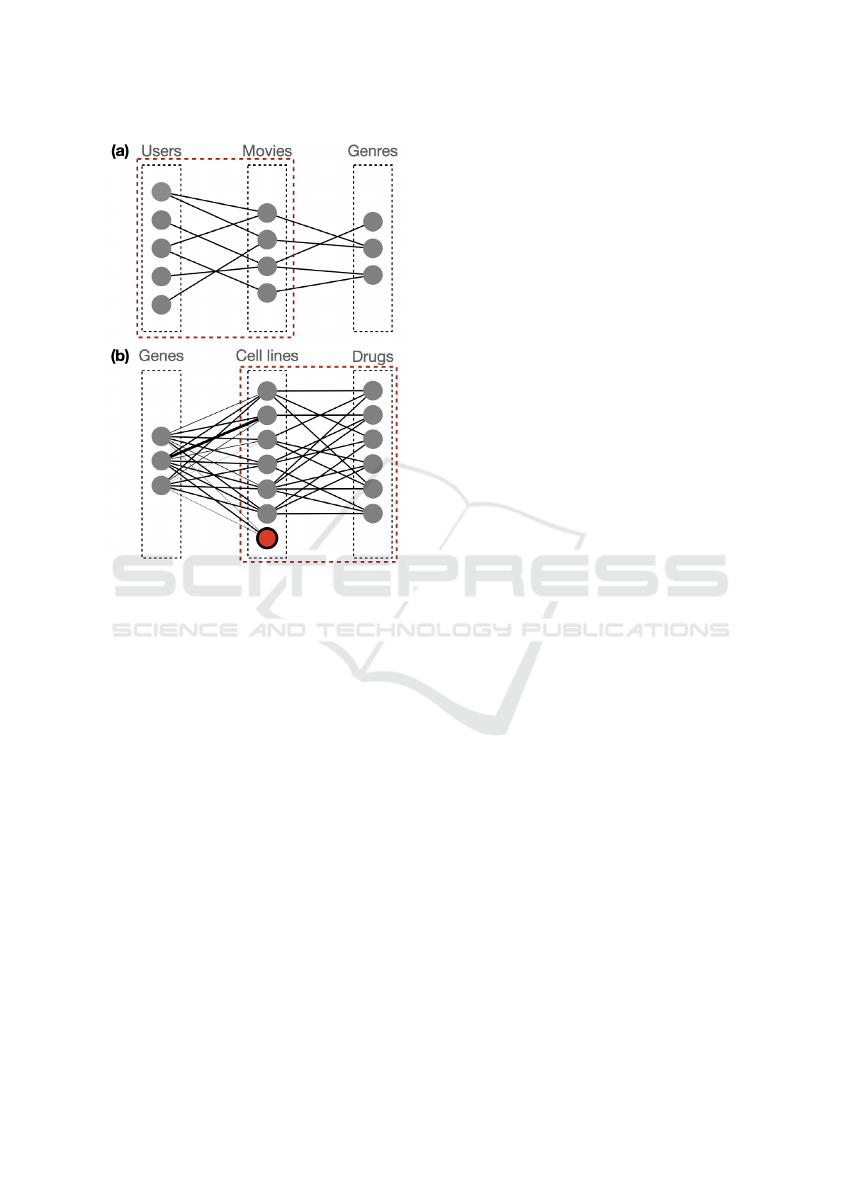
Figure 4: Sketch of the k-partite graphs. (a) represents the
USER-MOVIE-GENRE; both matrices are non-fully con-
nected and the connections are not weighted. (b) represents
the GENE-CELL-DRUG; in this case the association ma-
trix between genes and cell lines is dense and weighted. The
cell line in red, represents the new cell line for which only
connections with genes are known. In both sub-figures the
graph in the red box is the one on which we want to predict
unknown links.
4.7 Choosing the Number of Topics
There is no systematic method to specify the number
of topics, and this must be done empirically during
the training phase. A method which can be used is to
compute the AUROC curve for different numbers of
topics, and choose the number of topics which gives
the best performance.
5 APPLICATIONS
Here, we evaluate the proposed method on two sce-
narios. In the first case we have a graph USER-
MOVIE-GENRE and we show how the additional in-
formation MOVIE-GENRE is beneficial in link pre-
diction between USERS and MOVIES.
In the second case we apply our method to a
dataset GENE-CELL-DRUG. Here we simulate a dif-
ferent scenario: we suppose a new element is added to
the CELL partition. Moreover, such element does not
have any connection with any element in DRUG par-
tition, but only connection with elements in GENE.
We prove that the links in the GENE-CELL layer of
the graph is enough to effectively predict links in the
CELL-DRUG dataset for the newly inserted elements.
5.1 Application to a Movie Dataset
This dataset mimics a classic user-product dataset
where the link prediction is performed for recommen-
dation purposes and the additional information are
available regarding each of the products.
Dataset: the dataset is sketched in panel(a) of Fig-
ure 4. In a crowd sourced research we collected a
dataset of 130 users, each of who indicates among a
set of 66 movies which ones they have watched at.
Each movie is also linked to one or more genre, in a
set of 19 possible genres. In the dataset we have a
total of 1568 connections between users and movies
and 230 connections between movies and genre.
Evaluation: first of all, for the target association
matrix R
UM
between users and movies, we create an
associated mask matrix M of the same dimension. A
random 5% of the element of M are 0, while the oth-
ers are ones. Then we compute an association matrix
R
′
UM
, equal to the component-wise multiplication of
R
UM
and M. Thus, for any zero-entry of M, the cor-
responding entry in R
′
UM
will be set to 0. This corre-
spond to the deletion of some edges in the network.
Successively, we run PLSA using R
′
UM
and in order
to predict novel edges. The predictions made by the
system are the probability of edges being generated.
On the portion corresponding to the mask coefficients
equal to 0 we compute two measures, namely the Av-
erage Precision Score (APS) and the Area Under the
Receiver Operating Characteristic curve (AUROC).
We run this test several times, varying the matrix M.
For each run the performance is recorded. The final
performance is the mean performance averaged over
all the runs.
Number of Topics: To determine the number of top-
ics to use, one should be
In order to evaluate the benefits that can derive
from the inclusion of the second graph layer between
movies and genres, we run the algorithm twice: once
with the bipartite graph and once with the 3-partite
graphs, and we compared the performances. Results
are reported in Figure 5. The results demonstrate that
our method is effectively able to exploit and propa-
gate the information of the auxiliary graph and, thus,
KDIR 2022 - 14th International Conference on Knowledge Discovery and Information Retrieval
134
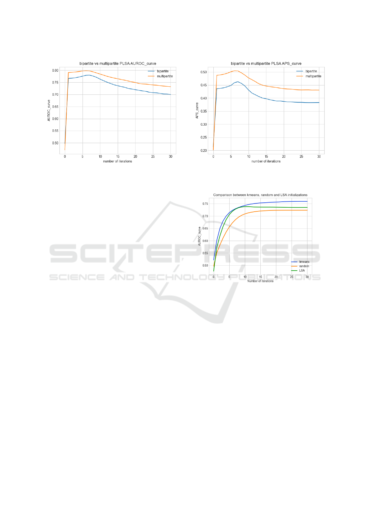
(a) Area under the ROC curve. (b) Average Precision score.
Figure 5: Results of the first use case. The plots shows that the addition of the second matrix is able to improve the results of
both AUROC and APS of approximately the 10%.
is a valuable method for link prediction in k-partite
graphs.
5.2 Application to a Drug Dataset
Here we test our method on a biological dataset about
the response of tumoral cell lines (biological model
employed in in vitro experiments) to anti tumor drugs.
Dataset: Given a cell line, it can be either sensitive
or resistant to a certain drug. Furthermore, each cell
line is also associated with a panel of genes, and for
each cell line and each gene the link connecting the
two has a weight that represent the expression (level
of activity) of the gene in the cell line. The topology
of the graph is depicted in Figure 4, panel (b). We
have a set of 576 genes, a set of 379 cell lines and a
set of 202 drugs. The graph connecting genes to cell
lines is dense and weighted, while the other is sparse
and unweighted.
Evaluation: on this dataset we performed two types
of evaluation. First of all we compared the AUROC
accordingly to the type of initialization. We did this
test by using a 5% mask on the cell line to drugs ma-
trix, as in the previous experiment. Results are re-
ported on Figure 6. We can observe that the random
initialization is the worse, while the k-means based
one performs the best and allows to obtain an AUROC
greater than 75% after only 10 iterations.
In second type of experiment, we supposed to add
a cell line to the dataset. For the given cell line the
gene expression (and thus the left graph) is known,
while the association to the drugs are not (refer to Fig-
ure 4. We simulate this scenario with a leave-one-out
validation, where at each iteration we removed all the
edges between the selected cell line and the drugs. We
measure the calculated the ROC curve for the experi-
Figure 6: Comparison of the AUROC with different initial-
ization strategies on the k-partite graph.
ment and we got a AUROC of 0.622. Results are re-
ported in Figure 7. Although a AUROC of 0.622 may
not impress, it has to be noted that all the predictive
power come from the supplementary graph layer (i.e.,
the cell to gene association); indeed, as there is no
previous information about the relationship between
the cell line and any of the drugs, only using the such
matrix let to a 0.5 of AUROC, which means that it is
not possible to predict anything.
6 CONCLUSION AND FUTURE
WORK
The PLSA is a method designed to work on corpus of
documents to extract from them relevant topics. Yet,
it can easily extended to work with bipartite graph for
the task of link prediction. However, extending PLSA
to work with k-partite graph is not trivial and requires
Generalization of Probabilistic Latent Semantic Analysis to k-partite Graphs
135

Figure 7: ROC curve of the leave-one-out experiment.
to modify the methods itself. In this work we de-
rived a version of PLSA which is able to work with
k-partite graphs as well with bipartite graphs, thus ex-
tending the potential of the method. Indeed, k-partite
graphs have shown to be valuable model for many dif-
ferent types of data, in particular in bioinformatics,
healthcare and recommender systems. In particular,
we firstly derived a new bayesian model that extends
the classical PLSA to k-partite graphs; then we de-
rived the Expectation-Maximization (EM) algorithm
to train the model from the data. Our proposed algo-
rithm is capable to deal with k-partite graphs of any
size, without limitation.
Through evaluation on two datasets, we show how
the extended PLSA is able to exploit information from
auxiliary graph’s layer to enhance the link prediction
in the main bipartite graph.
Future work comprise better evaluation of the
method and in particular of its variants (e.g., different
initializations, stop critera) and study on how to iden-
tify the best number of topics to guarantee optimal
performance. Furthermore we will apply the method
to real-world scenarios, such as the problem of drug
repurposing.
Finally, we plan to further investigate the proba-
bilistic properties of such method to propose an ex-
tension that is able to provide an explanation for each
predicted link, thus contributing in the direction of ex-
plainable artificial intelligence.
REFERENCES
Benchettara, N., Kanawati, R., and Rouveirol, C. (2010).
Supervised machine learning applied to link predic-
tion in bipartite social networks. In 2010 international
conference on advances in social networks analysis
and mining, pages 326–330. IEEE.
Boyd, S. and Vandenberghe, L. (2004). Convex Optimiza-
tion.
Ceddia, G., Pinoli, P., Ceri, S., and Masseroli, M. (2020).
Matrix factorization-based technique for drug repur-
posing predictions. IEEE journal of biomedical and
health informatics, 24(11):3162–3172.
Daud, N. N., Ab Hamid, S. H., Saadoon, M., Sahran, F., and
Anuar, N. B. (2020). Applications of link prediction
in social networks: A review. Journal of Network and
Computer Applications, 166:102716.
Dempster, A. P., Laird, N. M., and Rubin, D. B. (2015).
Maximum likelihood from incomplete data via the em
algorithm.
Dissez, G., Ceddia, G., Pinoli, P., Ceri, S., and Masseroli,
M. (2019). Drug repositioning predictions by non-
negative matrix tri-factorization of integrated associa-
tion data.
Farahat, A. and Chen, F. (2015). Improving probabilistic la-
tent semantic analysis with principal component anal-
ysis.
Gligorijevi
´
c, V., Malod-Dognin, N., and Pr
ˇ
zulj, N. (2016).
Patient-specific data fusion for cancer stratification
and personalised treatment. In Biocomputing 2016:
Proceedings of the Pacific Symposium, pages 321–
332. World Scientific.
Haugh, M. (2015). The em algorithm.
Hofmann, T. (1999). Probabilistic latent semantic analysis.
Hofmann, T. and Puzicha, J. (1998). Unsupervised learning
from dyadic data.
Hong, L. (2012). Probabilistic latent semantic analysis.
Hwang, T., Atluri, G., Xie, M., Dey, S., Hong, C., Kumar,
V., and Kuang, R. (2012). Co-clustering phenome–
genome for phenotype classification and disease gene
discovery. Nucleic acids research, 40(19):e146–e146.
Koptelov, M., Zimmermann, A., Cr
´
emilleux, B., and
Soualmia, L. (2020). Link prediction via community
detection in bipartite multi-layer graphs. In Proceed-
ings of the 35th Annual ACM Symposium on Applied
Computing, pages 430–439.
Kumar, A., Singh, S. S., Singh, K., and Biswas, B. (2020).
Link prediction techniques, applications, and perfor-
mance: A survey. Physica A: Statistical Mechanics
and its Applications, 553:124289.
Kumar, P. and Sharma, D. (2020). A potential energy and
mutual information based link prediction approach for
bipartite networks. Scientific Reports, 10(1):1–14.
Liu, Q., Long, C., Zhang, J., Xu, M., and Lv, P. (2021). Tri-
atne: Tripartite adversarial training for network em-
beddings. IEEE Transactions on Cybernetics.
Menon, A. K. and Elkan, C. (2011). Link prediction
via matrix factorization. In Joint european confer-
ence on machine learning and knowledge discovery
in databases, pages 437–452. Springer.
Pham, C. and Dang, T. (2021). Link prediction for biomed-
ical network. In The 12th international conference on
advances in information technology, pages 1–5.
Pinoli, P., Srihari, S., Wong, L., and Ceri, S. (2021). Iden-
tifying collateral and synthetic lethal vulnerabilities
within the dna-damage response. BMC bioinformat-
ics, 22(1):1–17.
KDIR 2022 - 14th International Conference on Knowledge Discovery and Information Retrieval
136

Thor, A., Anderson, P., Raschid, L., Navlakha, S., Saha, B.,
Khuller, S., and Zhang, X.-N. (2011). Link prediction
for annotation graphs using graph summarization. In
International Semantic Web Conference, pages 714–
729. Springer.
Zhang, L., Li, J., Zhang, Q., Meng, F., and Teng, W.
(2019). Domain knowledge-based link prediction
in customer-product bipartite graph for product rec-
ommendation. International Journal of Information
Technology & Decision Making, 18(01):311–338.
ˇ
Zitnik, M. and Zupan, B. (2014). Data fusion by matrix
factorization. IEEE transactions on pattern analysis
and machine intelligence, 37(1):41–53.
A THE EM ALGORITHM
In this section, we present the general framework of
the EM algorithm (Haugh, 2015), (Dempster et al.,
2015). We are given a vector of observation x, as well
as a parameter θ which we want to estimate through
the maximization of the likelihood function. The ini-
tial problem is therefore :
max
θ
l(x, θ)
where l is the log likelihood of the problem. The
EM algorithm is used when solving this optimization
problem is difficult. The way it is built is by introduc-
ing a vector z of latent random variables. These ran-
dom variables provide additional information about
the data. The problem is that they are not observed.
What the EM-Algorithm does is it computes simul-
taneously the correct value of θ and of z. Given an
estimate of the parameter θ
(p)
, the way θ
(p+1)
is com-
puted is through two steps : The E-Step and the M-
Step. the algorithm is given as an entry a first guess
of θ. It runs the E-Step, then the M-Step, and does so
for a fixed number of iterations.
A.1 The E-Step
The E-Step corresponds to the estimation of the dif-
ferent latent random variables (or rather their proba-
bility distribution). The end result of this step is the
computation of a function Q(θ), whose probabilistic
expression is:
Q(θ) = E(l(θ, x, z)|x, θ
(p)
)
Where l(θ, x, z) is the log-likelihood of both the set of
observed and latent variables. Note that the expres-
sion of l(θ, x, z) is different of l(x, θ), and this is why
the EM algorithm works. Being able to compute Q is
usually equivalent to the computation of the following
probabilities :
P(z|x, θ
(p)
)
A.2 The M-Step
The M-Step corresponds to the next estimation of the
parameter θ. The M-Step computes θ
(p+1)
by solving
the following optimization problem:
max
θ
Q(θ)
This optimization problem is often much simpler than
the original problem, and it is often the case that
analytical expressions of θ
(p+1)
can be found (as in
PLSA).
A.3 Link with PLSA
To make matters clearer, we map the variables in-
volved in PLSA with the general framework of the
EM-algorithm:
• x : The association matrices R
i, j
• z: the indicator variables z(t, v, w), which equal 1
if topic t has been chosen for edge (v, w); 0 other-
wise, for each k ∈ [1, ..., K], (v, t) ∈ V
k
× T
• θ: The probability matrices P(v|t), P(t|(i, j)), for
each k ∈ [1, ..., K], (v, t) ∈ V
k
× T , (i, j) ∈ A .
Generalization of Probabilistic Latent Semantic Analysis to k-partite Graphs
137
