Semi Real-time Data Cleaning of Spatially Correlated Data in Trafﬁc

Sensor Networks

Federica Rollo

, Chiara Bachechi

and Laura Po

“Enzo Ferrari” Engineering Department, University of Modena and Reggio Emilia, Italy

Keywords:

IoT, Trafﬁc Model, Anomaly Detection, Sensor Faults, Big Data Streams, Correlation, Correlated Sensors.

Abstract:

The new Internet of Things (IoT) era is submerging smart cities with data. Various types of sensors are

widely used to collect massive amounts of data and to feed several systems such as surveillance, environmental

monitoring, and disaster management. In these systems, sensors are deployed to make decisions or to predict

an event. However, the accuracy of such decisions or predictions depends upon the reliability of the sensor

data. By their nature, sensors are prone to errors, therefore identifying and ﬁltering anomalies is extremely

important. This paper proposes an anomaly detection and classiﬁcation methodology for spatially correlated

data of trafﬁc sensors that combines different techniques and is able to distinguish between trafﬁc sensor

faults and unusual trafﬁc conditions. The reliability of this methodology has been tested on real-world data.

The application on two days affected by car accidents reveals that our approach can detect unusual trafﬁc

conditions. Moreover, the data cleaning process could enhance trafﬁc management by ameliorating the trafﬁc

model performances.

1 INTRODUCTION

Public Administrations have begun to capture the

large amount of data collected through IoT sensors

in order to face the big challenge of sustainable de-

velopment. Nowadays, many cities are equipped with

trafﬁc sensors installed on their road networks. The

most diffuse sensor type is the induction loop: static

sensors that are embedded under the road surface and

provide real-time vehicle count and speed estimation.

These data can be used as input to simulate real-

time trafﬁc scenarios that can effectively help Public

Administration to cope with the mobility challenge

– and instantaneously optimizing the transportation

ﬂow while sending new instructions to smart city de-

vices like trafﬁc lights. Trafﬁc sensors are of great

value for urban trafﬁc modeling. However, they are

not free of errors and faults, and the degradation of

sensor performance can heavily affect the output of

trafﬁc model (Bachechi et al., 2020c). Therefore, de-

tecting faulty trafﬁc sensors is a fundamental step in

order to boost the quality of the trafﬁc management

system (Bachechi et al., 2020d; Bachechi et al., 2021;

Bachechi et al., 2022a; Desimoni et al., 2020). On the

https://orcid.org/0000-0002-3834-3629

https://orcid.org/0000-0003-2323-0573

https://orcid.org/0000-0002-3345-176X

other hand, anomalies in trafﬁc sensor observations

can also derive from non-conventional trafﬁc condi-

tions such as accidents, slowdowns, or street closures,

representing a consequent change in the environment.

Road trafﬁc congestion causes a waste of time and

money, promptly assessing the occurrence of trafﬁc

anomalies can minimize the impact and duration of a

road accident and the resulting trafﬁc congestion. The

ﬁrst step to assess the imminent emergence of car ac-

cidents is to detect deviations from normal trafﬁc pat-

terns.

The goal of this paper is to deﬁne an anomaly

detection and classiﬁcation methodology that can be

applied to massive trafﬁc data streams in semi-real-

time. Our approach can be applied to trafﬁc sensors

that measure both ﬂow and speed. The methodology

is discussed and applied in a real scenario, the traf-

ﬁc sensor network of Modena, an Italian city in the

Emilia-Romagna region.

The rest of this paper is structured as follows: Sec-

tion 2 describes related work, while the methodology

is detailed in Section 3. The use case and the conﬁg-

uration of the data cleaning process are discussed in

Section 4. Section 4.3 describes the results obtained

and the comparison with real trafﬁc conditions under-

lined in newspapers on two different days. Conclu-

sions and future work are sketched in Section 5.

Rollo, F., Bachechi, C. and Po, L.

Semi Real-time Data Cleaning of Spatially Correlated Data in Trafﬁc Sensor Networks.

DOI: 10.5220/0011588500003318

In Proceedings of the 18th International Conference on Web Information Systems and Technologies (WEBIST 2022), pages 83-94

ISBN: 978-989-758-613-2; ISSN: 2184-3252

2 RELATED WORK

Anomaly detection in time-series is a research area of

data science and machine learning that has received

much attention. With sensors pervading our everyday

lives, we see an exponential increase in the availabil-

ity of streaming, time-series data. In the literature, we

ﬁnd supervised, unsupervised, and semi-supervised

anomaly detection algorithms (G

ornitz et al., 2012;

Ramchandran and Sangaiah, 2018). However, several

methods are formerly created for processing data in

batches, and unsuitable for real-time streaming appli-

cations.

Several techniques have also been employed in

the context of sensor fault detection (Zamini and

Hasheminejad, 2019; Zhang et al., 2020; Chan-

der and Kumaravelan, 2022; O’Reilly et al., 2014).

ARIMA (Autoregressive Integrated Moving Average)

is a general-purpose technique effective at detecting

anomalies in data with regular daily or weekly pat-

terns. Extensions of ARIMA enable the automatic

determination of seasonality. ARIMA has also been

applied in the context of trafﬁc anomaly detection

that considers imbalanced, non-stationary properties

of the trafﬁc sensor network (Yu et al., 2016; Zare

Moayedi and Masnadi-Shirazi, 2008), and it showed

remarkable detection precision and real-time perfor-

mance. In (Kurian et al., 2015), a system to auto-

matically diagnose faults in induction loop sensors

measurements is described. The system is based on

an impulse test and thus requires to develop an em-

bedded circuit. In this paper, we will focus on au-

tomatic fault recognition methodologies that do not

require any embedded system. A possible approach

is described in (Zygouras et al., 2015); in this study,

faulty readings from trafﬁc sensors are identiﬁed by

examining the correlations among them and by taking

advantage of the ubiquitous citizens through crowd-

sourced data. The authors evaluate cross-correlation

between sensors using the Pearson metric, and then

employing a multivariate ARIMA model to detect

anomalies considering the correlated sensors. Mosh-

taghi et al. (Moshtaghi et al., 2011) proposed a

clustering method called Forgetting Factor Iterative

Data Capture Anomaly Detection (FFIDCAD) for on-

line anomaly detection on normal data. The novel

approach of FFIDCAD inspired the development of

other algorithms for the identiﬁcation of events in sen-

sor network (Ali et al., 2015).

From the best of our knowledge, ARIMA has

never been tested in combination with FFIDCAD in

the context of trafﬁc anomalies detection, nor in com-

bination with the correlation among trafﬁc sensors;

our paper is a new example of this combination.

3 METHODOLOGY

Trafﬁc sensors measurements are multivariate spatial

time series, since they provide information about two

variables: the trafﬁc ﬂow and the average speed of

vehicles. Besides, the two variables are not indepen-

dent: the number of vehicles and their average speed

are correlated. The methodology we developed to de-

tect anomalies and distinguish between sensor faults

and unusual trafﬁc conditions is composed of three

steps:

• Studying the Correlation among Trafﬁc Sensors:

this phase consists of an analysis of the sensor

network. The scope is to identify groups of traf-

ﬁc sensors whose measurements are correlated

by studying historical time series, as described

in (Bachechi et al., 2022b). Two sensors are

considered correlated if their Detrending Cross-

Correlation Analysis Coefﬁcient (DCCA) corre-

lation coefﬁcient is higher or equal to 0.7 in an in-

terval of one hour and their distance is lower than

2500 meters.

• Anomaly Detection: abnormal observations that

deviate from the vast common behavior of the sen-

sors are discovered for each sensor.

• Anomaly Classiﬁcation: anomalies are classi-

ﬁed as sensor faults or unusual trafﬁc conditions.

In (Bachechi et al., 2022b), the classiﬁcation

methodology is described in detail. Each anomaly

is associated with anomalies identiﬁed in an adja-

cent time interval. The amplitude of this time in-

terval should be deﬁned considering the frequency

of observations. Anomalies occurring in adjacent

time intervals in correlated sensors are consid-

ered unusual trafﬁc conditions. The anomalies ob-

served for sensors with a low number of correlated

sensors are more likely to be classiﬁed as sensor

faults. For this reason, for each anomaly classiﬁed

as sensor fault, the distance between the sensor it

belongs to and each trafﬁc sensor showing a si-

multaneous anomaly was evaluated. If there are at

least two other sensors experiencing an anomaly

in a radius of 1500 meters, the anomaly is classi-

ﬁed as an unusual trafﬁc condition. The remaining

anomalies are sensor faults.

In the following sections, we describe in detail the

techniques employed for anomaly detection.

3.1 Anomaly Detection Techniques

Anomaly is deﬁned as a point in time when the behav-

ior of the system is unusual and signiﬁcantly differ-

ent from previous, normal behavior (Chandola et al.,

WEBIST 2022 - 18th International Conference on Web Information Systems and Technologies

2008). The most common way to detect anomalies is

by modeling the average trend of data and detecting

deviations from the trend. We are interested in tech-

niques that allow detecting anomalies in real-time or

semi real-time. We identiﬁed three techniques to ﬁnd

anomalies on the trafﬁc sensors data streams. Firstly,

the ﬂow-speed correlation ﬁlter is applied to remove

the ﬂow and speed values that seem inconsistent if

considered related to one another. The ﬁlter was de-

scribed in detail in (Bachechi et al., 2022b) and is

based on the idea that, in a ﬁxed time interval, there

is a maximum number of vehicles that can pass on a

road at a certain speed. Other anomalous measure-

ments can be detected by combining the FFIDCAD

model and the ARIMA model.

FFIDCAD. is an iterative and multivariate anomaly

detection algorithm (Moshtaghi et al., 2011). This al-

gorithm assumes the data ﬁt the multivariate normal

distribution and exploits the correlation among differ-

ent features of data to identify the anomalies. The el-

ements of the input dataset are multidimensional fea-

ture vectors. The scope is to ﬁnd a set of clusters

that group the elements of the dataset. The bound-

ary of the clusters are deﬁned by hyperellipsoids. The

algorithm employs a continuous learning strategy to

estimate the hyperellipsoidal shape that covers the

data incrementally; each iteration of the algorithm ad-

justs the hyperellipsoidal model based on the mea-

surements up to the current time. The values of mean,

standard deviation, and covariance of the correlated

features are used to build the hyperellipsoids. The

out of the bound instances are classiﬁed as anomalous

data. At iteration k, the elements in the hyperellipsoid

are deﬁned by the formula:

ell

, S

−1

, t) = {x ∈ R

| (x−m

)

−1

(x−m

) ≤ t

}

where m

is the array containing the mean of the fea-

tures, x is the current data point, and S

−1

is the pre-

cision matrix, i.e., the inverse of the covariance. The

diagonal elements of the matrix measure how the vari-

ables are clustered around the mean, while the off-

diagonal elements express the independence of the in-

put features. t

is the conﬁdence space of the data dis-

tribution, i.e., the range of values that we expect to be

non-anomalous. The statistical p-value is used to de-

ﬁne the conﬁdence space. For example, if p = 0.98,

then the ellipsoid will cover the 98% of the data. In

other words, a data point has 98% probability to be an

acceptable value (near to the mean of the sample). p

should be set based on the assumption that anomalies

are rare in the dataset. In trafﬁc sensors, the correlated

features for the deﬁnition of the hyperellipsoids are

ﬂow and speed. The detailed analysis of sensor data

provided in (Bachechi et al., 2022b) reports that traf-

ﬁc data are non-stationary time series. To increase the

tracking capabilities of the model in non-stationary

environments, a forgetting factor λ ∈ (0, 1) was in-

troduced when updating the parameters of the model.

The mean is updated incrementally by the formula:

= λm

k−1

+ (1 − λ)x

At iteration k + 1, the precision matrix is updated as:

−1

k+1

−1

k − 1

[I −

k+1

− m

)(x

k+1

− m

)

−1

+ (x

k+1

− m

)

−1

k+1

− m

)

]

ARIMA. is a statistical method for time series anal-

ysis and forecast. It is able to model temporal data

with seasonality and allows capturing a set of stan-

dard temporal structures in time series data to forecast

new data (Bianco et al., 2001). For anomaly detection

purposes, a model of the sample time series is built,

then the anomalies are identiﬁed by comparing the

forecast with the real data. ARIMA combines an au-

toregression (AR) model and a moving average (MA)

model, and it is integrated (I), which means it exploits

the differencing technique to make stationary the non-

stationary time series. Indeed, like all the regression

models, also the ARIMA model can be applied to

non-stationary time series only after making it station-

ary since trends negatively affect the model. The AR

model identiﬁes the dependent relationship between

an observation and a variable number of lagged ob-

servations. This dependency is explained by the fol-

lowing formula:

= α + β

t−1

+ β

t−2

+ ... + β

t−p

+ ε

where Y

t−1

is the ﬁrst lag of the series, β

is its coef-

ﬁcient estimated by the model and α is the intercept

term. On the other hand, the MA model detects the

dependency between an observation and the lagged

forecast errors ε

caused by the autoregressive model,

following the formula:

= α + ε

+ ω

t−1

+ ω

t−2

+ ... + ω

t−p

The model exploits three conﬁguration parameters: p,

the lag order, i.e., the number of lag observations in-

cluded in the autoregressive model, d, the degree of

differencing, i.e., the number of times the raw obser-

vations are differenced to achieve stationary and to

remove any seasonality or trends, and q, the order

of moving average, i.e., the number of lagged fore-

cast errors for the prediction. To ﬁnd the parameters

which ﬁt better the sampled data, an iterative process

can be set up for building multiple models with differ-

ent parameters and checking the result. The Python

implementation of ARIMA in the statsmodels library

Semi Real-time Data Cleaning of Spatially Correlated Data in Trafﬁc Sensor Networks

Figure 1: Overview of the data cleaning process.

allows discovering the optimal conﬁguration parame-

ters for each model automatically. Therefore, it is not

necessary to ﬁnd these values with manual tests.

3.2 Data Cleaning Process

The anomaly detection techniques are combined in a

complex data cleaning process, as illustrated in Fig-

ure 1. Firstly, data coming from sensors are ﬁltered

through the ﬂow-speed correlation ﬁlter. The “ﬁl-

tered” observations are replaced by the average of the

reliable proximal observations. The resulting mea-

surements are given as input to the FFIDCAD model;

then, the model results are classiﬁed and divided into

sensor faults and unusual trafﬁc conditions consid-

ering the correlation between sensors. The obtained

collection of observations, labeled with anomaly clas-

siﬁcation, is then processed to remove sensor faults,

which are replaced with an average of proximal ob-

servations. Then, the obtained modiﬁed observations

are aggregated with a certain time interval and given

as input to the ARIMA model. Anomalies detected by

ARIMA are then classiﬁed, and the ﬁnal result is pro-

duced. The process is repeated for each trafﬁc sensor.

The anomaly detection techniques are employed

as complementary techniques to ﬁnd all the possible

anomalies. We were not expecting to ﬁnd a signiﬁcant

intersection between the anomalies found by the dif-

ferent techniques. However, to verify this assumption,

we compare the anomalies found by the ﬂow-speed

correlation ﬁlter, and by ARIMA and FFIDCAD on

a subset of real-world trafﬁc sensor data. We no-

ticed that the anomalies discovered by the ﬂow-speed

correlation ﬁlter were not detected by the FFIDCAD

model. This happens because FFIDCAD works on

the correlation between ﬂow and speed, but it does not

know the meaning of the values and the constraint of

their relationship. In conclusion, the ﬂow-speed cor-

relation ﬁlter cannot be replaced by FFIDCAD; it is a

complementary technique. Comparing the results of

FFIDCAD and ARIMA, we observed that only a low

percentage (less than 0.04%) of the total number of

sensor faults and unusual trafﬁc conditions detected

by the two techniques have been identiﬁed by both of

them.

This was evidence of the complementing behav-

ior of the methods. We conclude that all the methods

have to be applied to the sensor measurements since

there is not a signiﬁcant overlap.

4 USE CASE

Our methodology has been applied to the road traf-

ﬁc sensor network in the city of Modena. Around

400 trafﬁc sensors (induction loops) are spread in dif-

ferent locations of the city, in a single lane of the

street, usually near trafﬁc lights.

The sensors mea-

sure in real-time the number of vehicles (ﬂow) and

their average speed with a certain frequency. Sen-

sors data are collected into a PostgreSQL database

and exploited to emulate real routes of vehicles in

an urban trafﬁc model (Po et al., 2019b; Po et al.,

2019a; Bachechi et al., 2020c; Bachechi et al., 2020a;

Bachechi and Po, 2019). The frequency of mea-

surement is 1 minute for sensors located in urban

roads and 15 minutes for sensors in provincial area.

From September 2018 till April 2022, the database

collected more than 550 million trafﬁc observations.

Since trafﬁc sensors are installed under the surface of

the street, their maintenance cannot be continuously

granted, and sensors can be faulty and provide erro-

neous information. Thus, an anomaly detection pro-

cess is essential for two reasons: excluding outliers

from the trafﬁc model input and discovering unusual

trafﬁc conditions.

In the next subsections, we discuss the conﬁgura-

tion of the data cleaning process to ﬁt our use case.

4.1 Aggregation of the Input Data

The three implemented anomaly detection techniques

are applied to the measurements of each sensor sep-

Modena Sensor Map: https://trafair.eu/

modenasensormap/

WEBIST 2022 - 18th International Conference on Web Information Systems and Technologies

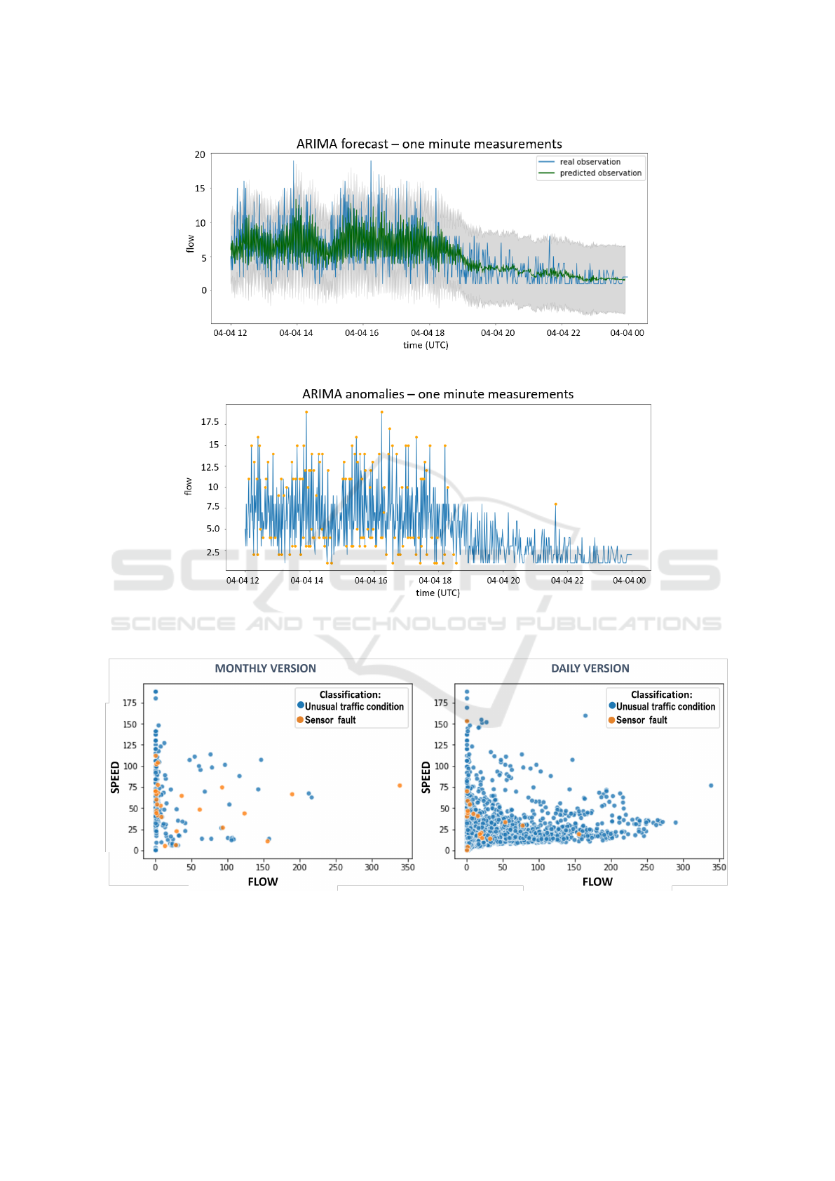
(a) Time series representing the measurements of the sensor (blue line) and the prediction of ARIMA (green line).

(b) Anomalies (orange points) detected by ARIMA.

Figure 2: ARIMA applied to one minute measurements of one sensor in some days of April 2019.

Figure 3: FFIDCAD anomaly detection over the whole month of November 2018 (monthly version) and the only 8

Novem-

ber 2018 (daily version).

arately. The ﬂow-speed correlation ﬁlter has to be

applied to the measurements as they are provided by

the sensors, without aggregation, since the application

of the average speed could modify the result signiﬁ-

cantly. To probe this decision, we could consider two

measurements, each of them related to one minute

time interval, the ﬁrst with ﬂow = 1 and speed =

150 and the second with ﬂow = 50 and speed = 60.

Semi Real-time Data Cleaning of Spatially Correlated Data in Trafﬁc Sensor Networks

The ﬁrst measurement is considered non-anomalous

by the ﬁlter, while the second is an anomaly. The

weighted average of the two values of speed is cal-

culated by the formula:

weighted average speed

∑

i=1

( f low

∗ speed

)

∑

i=1

f low

where f low

and speed

are the values of ﬂow and

speed of the i

measurement. In this case, the

weighted average speed is around 62. The aggre-

gated measurement, considering the weighted aver-

age, would be detected as anomalous by the ﬁlter.

In conclusion, it is better to apply the ﬁlter to the

“raw” observations, i.e., data not aggregated, to avoid

excluding some data that are instead valid measure-

ments.

FFIDCAD and ARIMA have been applied to the

“raw” data and to the data aggregated every 15 min-

utes. When the data are aggregated, the values of

the ﬂow are summed up for sensors with 1 minute

frequency, since they represent the actual number of

vehicles in the time interval of one minute. The

weighted average is evaluated to obtain a representa-

tive value of average speed in the aggregated interval.

The results obtained by using different aggrega-

tion intervals were compared in order to deﬁne the

best choice for each anomaly detection technique.

Firstly, FFIDCAD was tested on the measurements of

one day (8

November 2018) with 388,800 observa-

tions. The total number of anomalies found by FFID-

CAD in data aggregated every 15 minutes is 2286. In-

stead, the number of detected anomalies on the same,

not aggregated input data, is 11358. By applying clas-

siﬁcation, the total number of sensor faults on aggre-

gated data is 19 (0.008%), a very low number,

and 77 (0.0067%) on not aggregated data. Con-

sidering another day (15

April 2019), the anomalies

detected aggregating data are 3618, and 61 of them

are classiﬁed as sensor faults; without the aggregation

of data, the total number of anomalies grew to 12,129

and the sensor faults are 414. FFIDCAD, as described

in Section 3.1, studies the correlation between speed

and ﬂow. When aggregating data every 15 minutes,

some anomalies cannot be detected since the relation-

ship between ﬂow and speed changes when evaluat-

ing the sum of the ﬂow and the weighted average of

the speed in 15 minutes. For this reason, FFIDCAD

should be applied to raw input data.

We also evaluated the application of ARIMA to

both the “raw” measurements and the measurements

aggregated by 15 minutes. We compared the results,

and we found out that the conﬁguration, which con-

siders the “raw” measurements, detects many anoma-

lies. Plotting these anomalies and analyzing the val-

ues of ﬂow and speed, they did not seem to be anoma-

lous values. An example is provided by Figure 2a

which represents the measurements of one trafﬁc sen-

sor on a day of April 2019 (the blue line) and the pre-

diction of ARIMA (the green line). The gray area is

delimited between the lower and upper bounds of pre-

diction found by the model. The measurements with a

ﬂow value outside this area are detected as anomalies.

Figure 2b highlights with orange points the measure-

ments considered as anomalies by the model. As can

be seen, many measures are anomalies, by the ways

they seem to be non-anomalous. We suppose this

erroneous behavior happens because the sensors we

consider are installed near trafﬁc lights; therefore, it is

very common the ﬂow value grows fast and then again

takes on lower values. Studying the “unsteady” trend

of the time series, the ARIMA model is not able to

predict the one-minute measurements in the right way.

Therefore, we decided to apply the ARIMA model to

measurements aggregated by 15 minutes.

4.2 Time Interval of Concern

While the ﬂow-speed correlation ﬁlter consider the

“raw” measurements once a time, FFIDCAD and

ARIMA are applied to a set of measurements related

to a certain time interval. For the FFIDCAD model,

this means that the model can take as input the mea-

surements related to periods of different lengths, i.e.,

one day, one week, one month, and so on. Mean,

standard deviation, and covariance are calculated on

the entire dataset provided as input. In this way, the

model ﬁnds anomalies based on the whole period. For

the ARIMA model, the different duration of the time

interval is related to the training set.

FFIDCAD algorithm was applied to the entire

month of November 2018 and then on a single day:

November 2018. The anomalies detected by the

algorithm trained on the entire month are different

from the ones detected by the same algorithm trained

only on November 8

. The total number of anomalies

detected in the whole month was 7226 and only 281

of them on November 8

(only 26 classiﬁed as sen-

sor faults). Instead, with a daily interval of applica-

tion, the detected anomalies for the only 8

Novem-

ber were 2286 (19 sensor faults). The reduction in

the number of sensor faults in the daily version is be-

cause more anomalies are detected w.r.t. the monthly

version and some of these anomalies are simultane-

ous with the one previously erroneously classiﬁed as

sensor faults and now classiﬁed as unusual trafﬁc con-

ditions. The two different intervals of application de-

tect different anomalies, only 185 anomalies were de-

tected by both the monthly and daily version. 21

of the 26 anomalies classiﬁed as sensor fault by the

WEBIST 2022 - 18th International Conference on Web Information Systems and Technologies

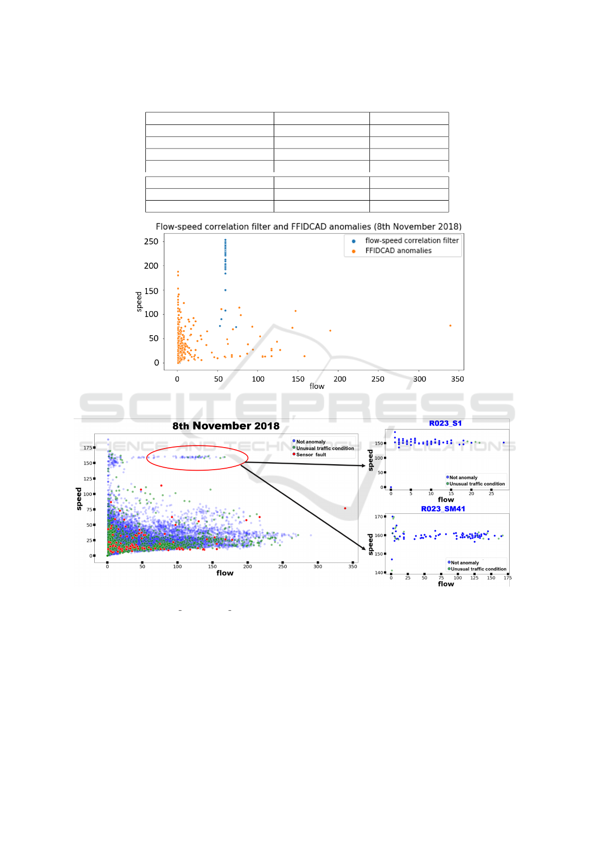
Table 1: Experimental results.

November 8

, 2018 April 15

, 2019

Available sensors 256 335

Raw measurements 383421 442802

Flow-speed ﬁlter anomalies 14076 (3.7% ) 14461 (3%)

FFIDCAD anomalies 11147 (3%) 16975 (4%)

FFIDCAD sensor faults 204 (0.02%) 2207(13%)

ARIMA anomalies 1431 (18%) 2485 (8%)

ARIMA sensor faults 96 (14.9%) 263 (9.5%)

Figure 4: Anomalies found by the ﬂow-speed correlation ﬁlter and the FFIDCAD model on the 8

November 2018.

Figure 5: Distribution of detected anomalies on the 8

November 2018 observed by all trafﬁc sensors and particulars for two

speciﬁc trafﬁc sensors (R023 S1 and R023 SM41).

monthly version are also detected by the daily ver-

sion. However, only 3 sensor faults detected by the

daily version are detected also by the monthly ver-

sion. In Figure 3, the difference between the anoma-

lies detected for all the sensors in the two versions

are represented in a two-dimensional space consider-

ing their ﬂow and speed. In this case, data are aggre-

gated every 15 minutes for both monthly and daily

versions. The reason why some anomalies are not

detected in the monthly version is that training the

model on the whole month means also considering

holidays and weekends that have a singular trend and

normally a lower ﬂow and can inﬂuence the detection

of anomalies in regular working days. For this reason,

we choose the daily version approach for FFIDCAD.

In the ARIMA model, instead, the train is made

on the entire month to predict one day. In this way,

different trends can be included in the model, i.e., the

Semi Real-time Data Cleaning of Spatially Correlated Data in Trafﬁc Sensor Networks

daily trend, but also the weekly trend, the different

behavior of the sensors in holidays, and so on. Thus,

the ARIMA model is used to predict sensor observa-

tions related to one day, but the model is trained on

the whole month.

4.3 Trafﬁc Accident Analysis

The application of our methodology was evaluated

on two speciﬁc days: 8

November 2018 and 15

April 2019. We selected these two days since there

were reported road accidents in streets controlled by

our sensors in Modena, so it was possible to check

if our methodology can distinguish between sensor

faults and unusual trafﬁc conditions. Table 1 reports

the number of available sensors, the number of ob-

servations, and the number and percentage of anoma-

lies detected by the different steps of the data cleaning

process for each of the two days.

In the ﬁrst experiment (on 8

November 2018)

the number of available sensors was lower than in the

second experiment; as a consequence, fewer observa-

tions were collected. The ﬂow-speed correlation ﬁlter

detects a similar percentage of anomalies in the two

days. In both experiments, the forgetting factor was

set to 0.999, as suggested by the authors of (Mosh-

taghi et al., 2011) and an FFIDCAD model was gen-

erated for each sensor. The time required by FFID-

CAD to ﬁnd anomalies is less than 1 second for each

sensor. Even if the percentage of detected anomalies

is similar in the two experiments, the percentage of

anomalies classiﬁed as sensor faults is signiﬁcantly

higher in the second experiment.

Figure 4 shows the anomalies found in the ﬁrst ex-

periment by the ﬂow-speed correlation ﬁlter and the

FFIDCAD model in a ﬂow-speed scatter plot. As

can be seen, most of the anomalies found by FFID-

CAD are related to low values of ﬂow, while the ﬂow-

speed correlation ﬁlter detects anomalies related to

very high values of speed.

Before applying the ARIMA model we replaced

the measurements ﬁltered by the ﬂow/speed corre-

lation ﬁlter and the ones identiﬁed as sensor fault

by FFIDCAD with the average of proximal measure-

ments. The ARIMA model was trained on the mea-

surements of the previous 30 days aggregated every

15 minutes to forecast the measurements of the next

hour. Then, the model was retrained with the real

measurements of the predicted hour to forecast the

next hour and so on. We used this approach to al-

low anomaly detection in real-time. The model re-

quires less than 10 minutes to predict the measure-

ments of the whole day. The percentage of anomalies

detected by the ARIMA model is halved in the second

experiment even if the absolute number of anomalies

is higher.

In the ﬁrst experiment, the anomalies classiﬁed as

sensor faults are related to 46 sensors, and the ones

classiﬁed as unusual trafﬁc conditions to 189 sensors.

While, in the second experiment, the anomalies clas-

siﬁed as sensor faults are related to 72 sensors, and

the ones classiﬁed as unusual trafﬁc conditions to 227

sensors.

All the aggregated measurements of all the avail-

able sensors on the 8

of November 2018 are dis-

played in Figure 5. It can be observed that the ma-

jority of sensor faults are detected when the speed

has low values. Moreover, the values with very high

speed and ﬂow (the ones indicated by the red circle)

appear to be anomalies observing the whole popu-

lation of sensors. The 96% of these measures with

speed higher than 150 km/h belongs to two sensors

(R023 S1 and R023 SM41). It was not possible to

identify their unrealistic measurements as anomalies

because anomaly detection is performed individually

for each sensor. Figure 7 displays the anomalies de-

tected in the second experiment. Like in the ﬁrst ex-

periment, the majority of sensor faults are detected

when the speed has low values. The values with very

high speed and ﬂow (the ones indicated by the red

circle) belong again to the two sensors R023 S1 and

R023 SM41. Since the majority of their observations

have high speed and ﬂow these sensors should be

checked to investigate the presence of malfunctions or

drifts. The data in the light-blue circle instead come

from another sensor’s observation, R009 SM19. This

sensor was not employed during the ﬁrst experiment

and shows always the same value of speed for very

different values of ﬂow; this suspect behavior needs

to be further analyzed. Therefore, our anomaly de-

tection methodology fails to detect a constant drift or

malfunction of the sensor that can emerge only when

its observations are compared with the ones of the

other sensors. On the 8

of November 2018, two re-

ported car accidents happened in Modena. We tested

the ability of our solution to detect accidents as un-

usual trafﬁc conditions. For each anomaly classiﬁed

as an unusual trafﬁc condition, an evidence score has

been evaluated. The evidence score is the number of

one-minute observations that were classiﬁed as un-

usual trafﬁc conditions by the FFIDCAD model in

the aggregated time interval. In Figure 6, the unusual

trafﬁc condition anomalies observed in sensors with a

distance from the accident location lower or equal to

1500 meters are displayed for each accident. The size

of the spots is proportional to their evidence score.

The two accidents occurred both at 03:30 PM UTC

in two different areas of the city, in the time interval

WEBIST 2022 - 18th International Conference on Web Information Systems and Technologies

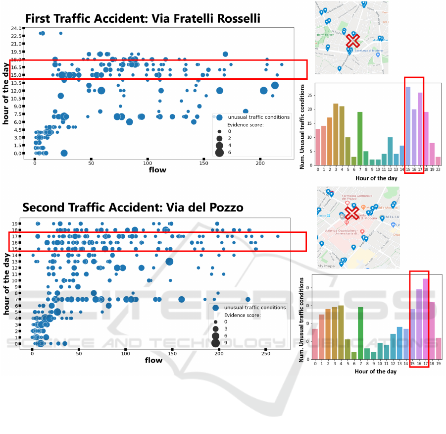
Figure 6: Distribution of the unusual trafﬁc conditions detected on the 8

November 2018 in sensor measurements near the

location of the car accident.

around that time (highlighted by red rectangles in Fig-

ure 6) we observe more unusual trafﬁc conditions in

sensors located nearby than in the other hours of that

day.

On 15

April 2019, there was one reported car

accident around 7 AM UTC. In Figure 8, the un-

usual trafﬁc conditions observed in the sensors with

a distance from the accident location lower or equal

to 1500 meters are displayed. The graph shows the

unusual trafﬁc conditions with a size proportional to

their evidence score evaluated considering the num-

ber of unusual trafﬁc conditions detected by the FFID-

CAD model at the same time interval. There are sev-

eral unusual trafﬁc conditions in the area around 6

AM in the moments preceding the accident. These

anomalies have a high evidence score and summing

the value of this score, the criticality of the trafﬁc con-

dition is evident.

Comparing Figure 6 to Figure 8 and also consider-

ing other plots of the same graph for a different group

of sensors, it is evident that our methodology can de-

tect slow-moving trafﬁc that usually interests morn-

ing and mid-afternoon hours. However, the relation

between slowdowns and car accidents should be fur-

ther analyzed to be able to successfully identify car

accidents.

5 CONCLUSION AND FUTURE

WORK

This paper has introduced a combined method for

the detection and classiﬁcation of anomalies on trafﬁc

sensors. Two anomaly detection algorithms, a ﬁlter-

ing technique, and an anomaly classiﬁer were com-

Semi Real-time Data Cleaning of Spatially Correlated Data in Trafﬁc Sensor Networks

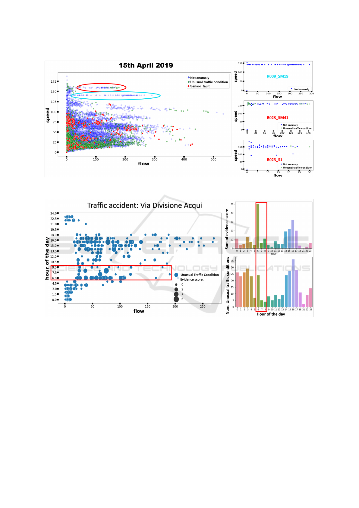
Figure 7: Distribution of detected anomalies the 15

April 2019 considering the ﬂow (number of vehicles in 15 minutes

interval) and speed (Km/h) observed by trafﬁc sensors.

Figure 8: Distribution of the unusual trafﬁc conditions detected on the 15

April in sensor measurements near the location of

the car accident.

bined to detect unusual trafﬁc conditions and sensor

faults. Sensor faults are observations collected from

induction loop sensors that should be discarded in or-

der to evaluate real trafﬁc data. Unusual trafﬁc condi-

tions, instead, provide useful information to detect de-

viations from trafﬁc trends and to identify critical situ-

ations such as car accidents. Having clean and correct

trafﬁc data is very important for the study and man-

agement of road trafﬁc; it also ameliorates the pre-

dictions of the trafﬁc ﬂows that can be generated us-

ing a trafﬁc model (Bachechi and Po, 2019; Po et al.,

2019a).

In the future, we will analyze the impact, on trafﬁc

model performance, of the detection and classiﬁca-

tion of anomalies on trafﬁc sensors. We plan to com-

pare the current implementation of the trafﬁc model

that uses all sensor data observations with a trafﬁc

model that uses a pre-processed input without sensor

faults. Moreover, we intend to implement the predic-

tion of trafﬁc congestion, thus exploiting multi-modal

data streams that combine the IoT data, weather con-

ditions, and social media data streams.

Detecting anomalies and sensor faults is an impor-

tant aspect of a wide variety of sensors used in smart

cities. The proposed anomaly detection methodol-

ogy for multivariate time series is designed for traf-

ﬁc sensors, but can be easily adapted for different

applications by modifying the ﬂow-speed ﬁlter con-

WEBIST 2022 - 18th International Conference on Web Information Systems and Technologies

sidering the given use case. As a future work, we

aim to deepen the problem of anomalies produced

by air quality monitoring sensors. Such sensors are

more sensitive to environmental changes than traf-

ﬁc sensors, their observations are strongly affected

by the values of humidity, temperature and also the

concentrations of other gases or particles (Rollo and

Po, 2021; Rollo et al., 2021; Bachechi et al., 2020b).

Moreover, air quality sensors are subject to rapid de-

terioration over time.

ACKNOWLEDGEMENTS

Research reported in this paper was partially sup-

ported by the TRAFAIR project 2017-EU-IA-0167,

co-ﬁnanced by the Connecting Europe Facility of the

European Union. The views and conclusions con-

tained in this document are those of the authors and

should not be interpreted as representing the ofﬁcial

policies, either expressed or implied, of the EU Com-

mission. The authors would like to thank in particular

the partners that contribute to the collection and man-

agement of trafﬁc sensor data: the City of Modena

and Lepida S.c.p.A..

REFERENCES

Ali, K., Anwar, T., Naqvi, I. H., and Jafry, M. H. (2015).

Composite event detection and identiﬁcation for wsns

using general hebbian algorithm. In 2015 IEEE In-

ternational Conference on Communications (ICC),

pages 6463–6468.

Bachechi, C., Desimoni, F., Po, L., and Casas, D. M.

(2020a). Visual analytics for spatio-temporal air qual-

ity data. In 2020 24th International Conference Infor-

mation Visualisation (IV), pages 460–466.

Bachechi, C., Desimoni, F., Po, L., and Casas, D. M.

(2020b). Visual analytics for spatio-temporal air qual-

ity data. In Banissi, E., Khosrow-shahi, F., Ursyn,

A., Bannatyne, M. W. M., Pires, J. M., Datia, N.,

Nazemi, K., Kovalerchuk, B., Counsell, J., Agapiou,

A., Vrcelj, Z., Chau, H., Li, M., Nagy, G., Laing, R.,

Francese, R., Sarfraz, M., Bouali, F., Venturini, G.,

Trutschl, M., Cvek, U., M

uller, H., Nakayama, M.,

Temperini, M., Mascio, T. D., Sciarrone, F., Rossano,

V., D

orner, R., Caruccio, L., Vitiello, A., Huang,

W., Risi, M., Erra, U., Andonie, R., Ahmad, M. A.,

Figueiras, A., Cuzzocrea, A., and Mabakane, M. S.,

editors, 24th International Conference on Information

Visualisation, IV 2020, Melbourne, Australia, Septem-

ber 7-11, 2020, pages 460–466. IEEE.

Bachechi, C. and Po, L. (2019). Implementing an urban

dynamic trafﬁc model. In Barnaghi, P. M., Gottlob,

G., Manolopoulos, Y., Tzouramanis, T., and Vakali,

A., editors, 2019 IEEE/WIC/ACM International Con-

ference on Web Intelligence, WI 2019, Thessaloniki,

Greece, October 14-17, 2019, pages 312–316. ACM.

Bachechi, C., Po, L., and Rollo, F. (2022a). Big data ana-

lytics and visualization in trafﬁc monitoring. Big Data

Res., 27:100292.

Bachechi, C., Rollo, F., Desimoni, F., and Po, L. (2020c).

Using real sensors data to calibrate a trafﬁc model for

the city of modena. In Ahram, T. Z., Karwowski,

W., Vergnano, A., Leali, F., and Ta

ıar, R., editors, In-

telligent Human Systems Integration 2020 - Proceed-

ings of the 3rd International Conference on Intelligent

Human Systems Integration (IHSI 2020): Integrating

People and Intelligent Systems, February 19-21, 2020,

Modena, Italy, volume 1131 of Advances in Intelligent

Systems and Computing, pages 468–473. Springer.

Bachechi, C., Rollo, F., and Po, L. (2020d). Real-time data

cleaning in trafﬁc sensor networks. In 17th IEEE/ACS

International Conference on Computer Systems and

Applications, AICCSA 2020, Antalya, Turkey, Novem-

ber 2-5, 2020, pages 1–8. IEEE.

Bachechi, C., Rollo, F., and Po, L. (2022b). Detection and

classiﬁcation of sensor anomalies for simulating urban

trafﬁc scenarios. Clust. Comput., 25(4):2793–2817.

Bachechi, C., Rollo, F., Po, L., and Quattrini, F. (2021).

Anomaly detection in multivariate spatial time series:

A ready-to-use implementation. In Mayo, F. J. D.,

Marchiori, M., and Filipe, J., editors, Proceedings of

the 17th International Conference on Web Informa-

tion Systems and Technologies, WEBIST 2021, Octo-

ber 26-28, 2021, pages 509–517. SCITEPRESS.

Bianco, A., Ben, M. G., Mart

ınez, E., and Yohai, V. (2001).

Outlier detection in regression models with arima er-

rors using robust estimates. J. Forecast., 20:565–579.

Chander, B. and Kumaravelan, G. (2022). Outlier de-

tection strategies for wsns: A survey. Journal of

King Saud University - Computer and Information

Sciences, 34(8):5684–5707. Cited By :3.

Chandola, V., Mithal, V., and Kumar, V. (2008). Compar-

ative evaluation of anomaly detection techniques for

sequence data. In Proceedings of the 8th IEEE Inter-

national Conference on Data Mining (ICDM 2008),

pages 743–748.

Desimoni, F., Ilarri, S., Po, L., Rollo, F., and Trillo-Lado,

R. (2020). Semantic trafﬁc sensor data: The trafair

experience. Applied Sciences, 10(17).

ornitz, N., Kloft, M., Rieck, K., and Brefeld, U. (2012).

Toward supervised anomaly detection. Journal of Ar-

tiﬁcial Intelligence Research (JAIR), 45.

Kurian, N., Thomas, A., and George, B. (2015). Automated

fault diagnosis in multiple inductive loop detectors.

11th IEEE India Conference: Emerging Trends and

Innovation in Technology, INDICON 2014.

Moshtaghi, M., Leckie, C., Karunasekera, S., Bezdek, J. C.,

Rajasegarar, S., and Palaniswami, M. (2011). Incre-

mental elliptical boundary estimation for anomaly de-

tection in wireless sensor networks. In Cook, D. J.,

Pei, J., Wang, W., Za

ıane, O. R., and Wu, X., editors,

11th IEEE International Conference on Data Mining,

ICDM 2011, Vancouver, BC, Canada, December 11-

14, 2011, pages 467–476. IEEE Computer Society.

Semi Real-time Data Cleaning of Spatially Correlated Data in Trafﬁc Sensor Networks

O’Reilly, C., Gluhak, A., Imran, M. A., and Rajasegarar,

S. (2014). Anomaly detection in wireless sensor net-

works in a non-stationary environment. IEEE Com-

mun. Surv. Tutorials, 16(3):1413–1432.

Po, L., Rollo, F., Bachechi, C., and Corni, A. (2019a). From

sensors data to urban trafﬁc ﬂow analysis. In 2019

IEEE International Smart Cities Conference, ISC2

2019, Casablanca, Morocco, October 14-17, 2019,

pages 478–485. IEEE.

Po, L., Rollo, F., Viqueira, J. R. R., Lado, R. T., Bigi,

A., L

opez, J. C., Paolucci, M., and Nesi, P. (2019b).

TRAFAIR: understanding trafﬁc ﬂow to improve air

quality. In 2019 IEEE International Smart Cities Con-

ference, ISC2 2019, Casablanca, Morocco, October

14-17, 2019, pages 36–43. IEEE.

Ramchandran, A. and Sangaiah, A. K. (2018). Chap-

ter 11 - unsupervised anomaly detection for high di-

mensional data—an exploratory analysis. In Sanga-

iah, A. K., Sheng, M., and Zhang, Z., editors, Com-

putational Intelligence for Multimedia Big Data on

the Cloud with Engineering Applications, Intelligent

Data-Centric Systems, pages 233 – 251. Academic

Press.

Rollo, F. and Po, L. (2021). Senseboard: Sensor mon-

itoring for air quality experts. In Costa, C. and Pi-

toura, E., editors, Proceedings of the Workshops of the

EDBT/ICDT 2021 Joint Conference, Nicosia, Cyprus,

March 23, 2021, volume 2841 of CEUR Workshop

Proceedings. CEUR-WS.org.

Rollo, F., Sudharsan, B., Po, L., and Breslin, J. G. (2021).

Air quality sensor network data acquisition, clean-

ing, visualization, and analytics: A real-world iot use

case. In Adjunct Proceedings of the 2021 ACM Inter-

national Joint Conference on Pervasive and Ubiqui-

tous Computing and Proceedings of the 2021 ACM In-

ternational Symposium on Wearable Computers, Ubi-

Comp ’21, page 67–68, New York, NY, USA. Associ-

ation for Computing Machinery.

Yu, Q., Jibin, L., and Jiang, L. (2016). An improved arima-

based trafﬁc anomaly detection algorithm for wireless

sensor networks. International Journal of Distributed

Sensor Networks, 12(1):9653230.

Zamini, M. and Hasheminejad, S. M. H. (2019). A compre-

hensive survey of anomaly detection in banking, wire-

less sensor networks, social networks, and healthcare.

Intell. Decis. Technol., 13(2):229–270.

Zare Moayedi, H. and Masnadi-Shirazi, M. A. (2008).

Arima model for network trafﬁc prediction and

anomaly detection. In 2008 International Symposium

on Information Technology, volume 4, pages 1–6.

Zhang, M., Guo, J., Li, X., and Jin, R. (2020). Data-driven

anomaly detection approach for time-series streaming

data. Sensors, 20(19):5646.

Zygouras, N., Panagiotou, N., Zacheilas, N., Boutsis, I.,

Kalogeraki, V., Katakis, I., and Gunopulos, D. (2015).

Towards detection of faulty trafﬁc sensors in real-time.

In MUD@ICML.

WEBIST 2022 - 18th International Conference on Web Information Systems and Technologies