
Increasing the Efficiency of Bolangi Substation Extension by Using
ACCC Conductor on 150 KV Sungguminasa-Bolangi Overhead
Power Line
Dendhy Widhyantoro
State Polytechnic of Jakarta, University of Indonesia, Jl. Prof. DR. G.A. Siwabessy Kampus, Depok, Indonesia
Keywords: Conductor Reconfiguration, ACCC, ACSR, Efficiency, Overhead Power Line, Substation.
Abstract: Electricity is one of the most important needs for society. Therefore, problems related to electricity will greatly
affect a country. An example of this problem is the electricity crisis. Electrical energy crisis may occur due to
lack of energy efficiency or high operating costs. One of the solutions to overcome these two problems is to
optimize several components that play a part in the distribution of electrical energy such as the conductors
used in the SUTT line. There are various types of conductors, including but not limited to ACSR and ACCC.
Switching to a higher performing conductor can contribute to solving this problem. There are several studies
that support replacing conductors with better ones can affect energy efficiency by increasing the power factor,
reducing power losses, and increasing transmission efficiency so that they can contribute to solving the
electrical energy crisis. The conductor that’s going to be used is ACCC, which is a conductor capable of
operating in high temperatures and has a low sag and is an upgrade and refinement of the ACSR conductor.
By doing this conductor reconfiguration process, the power factor of the substation increased by 6.59%,
transmission efficiency by 2.1% and reduced power loss by 52.82%.
1 INTRODUCTION
Electrical energy is an energy that is used by almost
all people. Therefore, it is one type of energy that is
extremely valuable, especially in the economic side
(Arismunandar & Kuwahara, 2004). Electricity crisis
in Indonesia is mostly related to economic problems,
such as the high operating costs at substations or the
lack of high energy efficiency on substations’ lines
which in turn may cause the aforementioned electrical
energy crisis. Energy efficiency in this case is defined
into more specific variables including but not limited
to; difference in power factor, difference in power
loss, and difference in transmission efficiency.
One of the possible solutions to solve this
electrical energy crisis problem is to optimize the
components that play a role in the distribution of
electrical energy such as the conductor that’s being
used. The conductors used in High Voltage Overhead
Lines (SUTT) play an important part in the
performance and efficiency of the system.
This research is conducted at the High Voltage
Overhead Lines of Sungguminasa – Bolangi where
there is a power loss of 0.2022 MW and a SAIFI index
of 0.57 which is high enough to cause a loss of
economic value. These problems are directly related
to the main component of the SUTT which is the
conductor. They can be of various types, including
but not limited to ACSR (Aluminum Conductor
Steel-Reinforced Cable) and ACCC (Aluminum
Conductor Composite Core).
ACSR is a type of conductor that has a high
capacity, high strain resistance (around 131.9 kN),
and is usually used on High Voltage Overhead Lines.
The outer strand is made of high purity aluminium
which results in good conductivity, light weight, and
low cost. The inner strand is made of steel which has
higher strength and inelastic deformation caused by
mechanical loads such as wind. Steel also has low
coefficient of thermal expansion under current load
(Kenge et al., 2016). These things make ACSR sag
much less than all-aluminium conductors (Lalonde et
al., 2018).
ACCC is a type of high-temperature low-sag
conductor which is capable of operating in high
temperatures and has a low sag. It’s an update or
improvement to ACSR. It replaces the steel core in
ACSR with carbon and glass fibre (Bryant, 2019).
This gives ACCC several advantages over ACSR.
Firstly, ACCC is capable of carrying twice as much
current as ACSR in general (Wareing, 2018).
466
Widhyantoro, D.
Increasing the Efficiency of Bolangi Substation Extension by Using ACCC Conductor on 150 KV Sungguminasa-Bolangi Overhead Power Line.
DOI: 10.5220/0011814100003575
In Proceedings of the 5th International Conference on Applied Science and Technology on Engineering Science (iCAST-ES 2022), pages 466-472
ISBN: 978-989-758-619-4; ISSN: 2975-8246
Copyright © 2023 by SCITEPRESS – Science and Technology Publications, Lda. Under CC license (CC BY-NC-ND 4.0)

Secondly, ACCC is lighter than ACSR, making it
possible for the saved weight to be used for additional
aluminium conductors. Thirdly, ACCC is softer than
ACSR. The latter may use stronger pure aluminium
which contributes to its tensile strength and improved
sag under icy load conditions, but it has less electrical
conductivity and has a limited operating temperature
and more power loss than ACCC (Chen et al., 2012).
Lastly, ACCC has a much smaller coefficient of
thermal expansion (CTE) of 1.6 ppm/C than ACSR.
This allows ACCC to operate at a much higher
temperature without excessive sag (Slegers, 2011).
Figure 1: Comparison of sag between ACSR and ACCC
conductor (Qiao et al., 2020).
Optimizing the conductor by reconfiguring it into
a higher performing one can help solve the problem
at Sungguminasa – Bolangi powerlines which is the
lack of energy efficiency. Therefore, based on the
advantages of ACCC over ACSR that have been
described above, the former is more suitable for usage
in High Voltage Overhead Lines as it will greatly help
with the energy efficiency issue that is being faced.
This study will calculate and compare the changes in
efficiency after executing the reconfiguration process
from ACSR conductor to ACCC on the High Voltage
Overhead Lines of Sungguminasa – Bolangi wherein
efficiency is again divided into several variables,
including power factor difference, power loss
difference, and transmission efficiency difference.
The purposes of this research will be divided into
three clear, concise points:
1. To calculate and compare the difference in
power factor before and after the conductor
reconfiguration process
2. To calculate and compare the difference in
power loss before and after the conductor
reconfiguration process
3. To calculate and compare the difference in
transmission efficiency before and after the
conductor reconfiguration process
2 THEORITICAL REVIEW
There are studies that discuss the use of several types
of conductors in substation lines. One of these studies
compares two types of conductors with different
specifications, one of them is the ACCC conductor
which has better specifications on a 150 kV
transmission system than the other conductor it’s
compared to. When compared, the ACCC conductor
has smaller resistance per phase and has larger
received power (MW) as well as larger current draw.
The author states that there’s an increase of 1.35% to
the efficiency (Handayani et al., 2019).
Another study discusses the conductor
reconfiguration process in the Mranggen Incomer
High Voltage Overhead Lines. The author states that
reconfiguration occurred because it utilized a single
phi system. Therefore, using this system may cause a
power outage if one of the lines is disturbed. Due to
this concern, they reconfigured the process into a
double phi system, followed by performing a series of
calculations based on the results. It was discovered
that the power loss in the Ungarang-Mranggen Line
before the reconfiguration process was 5.86 kW and
was reduced to 2.75 kW afterwards. Meanwhile, at
the Mranggen Incomer Ungaran-Purwodadi line, the
power loss was reduced from 13.39 kW to 8.9 kW
after reconfiguration (Imam G, 2017).
3 RESEARCH METHODS
This study uses multivariate data analysis technique
which is the method of processing a large number of
variables, where the aim is to find the effect of these
variables on an object simultaneously. The variables
that are analysed include the difference in
transmission efficiency, power factor, and power loss.
After these variables have been calculated before and
after the reconfiguration process, they will be
compared and analysed whether there is a relation
between variables or a relationship between several
variables with one variable (Wustqa et al., 2018).
3.1 Reconfiguration Method
The reconfiguration method is divided into several
steps, starting from de-energizing to installing the
conductor itself. The figure below shows the initial
condition of Bolangi 150 kV substation, without any
reconfiguration process done.
Increasing the Efficiency of Bolangi Substation Extension by Using ACCC Conductor on 150 KV Sungguminasa-Bolangi Overhead Power
Line
467
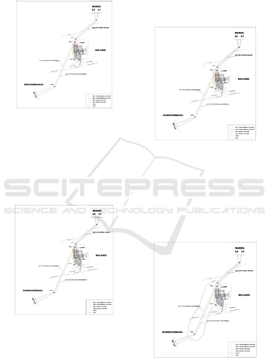
Figure 2: Substation’s starting condition.
Stage 1 starts with de-energizing Maros-Bolangi
#1 (Existing) line for 3 days to move conductor from
Maros #1 (Existing) bay line to Maros bay line
(New). Next is to re-energize Maros-Bolangi #1 via
the new bay line one day after de-energizing it.
Simultaneously, the relay distance at Maros #1 bay
line will also be replaced with a new differential relay
from new substation. After replacing the relay
distance, point to point operation will be carried out
to the RCC master station. After stage 1, the system
will look like what is depicted in the figure below.
Figure 3: Stage 1 of the conductor reconfiguration process.
Stage 2A starts with de-energizing Maros #1
(New) bay line, Sungguminasa #1 (Existing) bay line,
and 60 MVA bay transformer at 150 kV Bolangi
substation for one day to carry out the conductor
removal operation that’s located above the two
Bolangi substation busbars. After that, Maros-
Bolangi #1 will be re-energized via the new bay line
along with the 60 MVA bay transformer. Stage 2A is
shown in the figure below.
Figure 4: Stage 2A of the conductor reconfiguration
process.
Stage 2B first start with de-energizing Bolangi-
Sungguminasa #1 existing line again for 18 days
(continuation of stage 2A) to allow for the conductor
dismantling operation from T.Inc to T.112 and to do
a conductor stringing operation from T.112 to the new
gantry bay line of Sungguminasa #1 (New). After
that, the Sungguminasa-Bolangi #1 line will be
resuming operation via the new bay line. Also at this
stage, OPWG configuration is also carried out for 4
days after stage 2A. This stage is depicted in the
figure below.
Figure 5: Stage 2B of the conductor reconfiguration
process.
iCAST-ES 2022 - International Conference on Applied Science and Technology on Engineering Science
468

Next is stage 3 and 4. First, Sungguminasa-Maros
#2 (Existing) line is to be de-energized for sixteen
days to allow for the conductor dismantling operation
from T.111 to T.112 and conductor stringing
operation for the new conductor from T.111 to T.Out
and T.112 to T.Inc. Simultaneously, the relay distance
at Sungguminasa substation will also be replaced with
a differential relay. After that, Sungguminasa-
Bolangi #2 line will be operational. In stage 4,
transmission line will change to Bolangi-New Power
#2 line. Stage 3 and 4 are depicted together in the
figure below.
Figure 6: Stage 3 and 4 of the reconfiguration process.
Stage 5 is the conductor dismantling operation
and GSW T.76 – T.77 in Maros-Sungguminasa /
Bolangi #2 to T.01 Incomer New Power. OPGW
reconfiguration will also be done. After that, New
Power – Bolangi #2 line will be operational. Stage 6
is the last stage and it’s the installation and operation
of the new conductor in Maros-Sungguminasa. The
T.76 T/L Maros-Sungguminasa and TIP 01 New
Power incomer will be installed. After installation,
the New Power Line – Maros #2 will be operational.
This stage is shown in the figure below. Figure 8 also
shows the before and after of the reconfiguration
process with dotted lines indicating the before and
solid lines indicating the after.
Figure 7: Stage 6 of the conductor reconfiguration process.
Figure 8: Comparison of system before and after the
reconfiguration process.
4 RESULTS AND ANALYSIS
4.1 Results
Measurements of the observed variables for both
ACSR and ACCC conductors were taken and put
together into table 1 and table 2 respectively.
Increasing the Efficiency of Bolangi Substation Extension by Using ACCC Conductor on 150 KV Sungguminasa-Bolangi Overhead Power
Line
469

Table 1: Measurement results for ACSR conductor.
Measurement
Value
R (Resistance) (
0.1155
X
L
(Reactance) (
0.3064
A (Surface area) (mm
2
)
429.1
d (Conductor’s length) (km)
4.1
b (Air pressure) (mmHg)
756.06
T (Average temperature) ()
28
I (Current) (Ampere)
372
Q (Reactive power) (MVAR)
39.1
P (Power) (MW)
85.8105
E (Phase voltage) (Volt)
144
r (Radius) (mm)
28.62
D (Distance between wires) (m)
2.5
Table 2: Measurement results for ACCC conductor.
Measurement
Value
R (Resistance) (
0.0514
X
L
(Reactance) (
0.206
A (Surface area) (mm
2
)
546.5
d (Conductor’s length) (km)
4.1
b (Air pressure) (mmHg)
756.06
T (Average temperature) ()
28
I (Current) (Ampere)
387
Q (Reactive power) (MVAR)
25.2465
P (Power) (MW)
100.7348
E (Phase voltage) (Volt)
144
r (Radius) (mm)
14.315
D (Distance between wires) (m)
2.5
Firstly, resistance and reactance for both
conductors must be multiplied by the respective
conductors’ length.
(1)
(2)
After finding both resistance and reactance
values, we can find the impedance using Pythagoras
theorem and finding the phase by finding the arctan
of reactance over resistance.
(3)
(4)
Put the two values together, we get the total
impedance (Z):
(5)
First is to calculate the first variable which is the
power factor. From the two tables of ACSR and
ACCC measurements, we take the P (power) and the
Q (reactive power) of each conductor and find the S
(apparent power) and from there we can find the
power factor.
(6)
Plugging the apparent power into the power factor
formula, we get:
(7)
(8)
Second is to calculate the power loss which is
divided into two parts: transmission power loss and
corona power loss. Calculating transmission power
loss for 3 phase system is to multiply the current
squared with resistance and three.
(9)
Before we can find the corona losses, we need to
find the relative air density and the voltage
gradient (E
g
). We can find the relative air density
using the following formula:
(10)
To find the voltage gradient for a 3-phase
transmission line, we can use the formula from (W. S.
Peterson, 1933).
(11)
Finally, after calculating both relative air density
and voltage gradient, we can find the corona loss for
both conductors with the following formula which is
Peek’s formula and is based on an equation from (F.
W. Peek, 1929) to find the power loss due to the
corona effect (ionization surrounding the conductor).
Corona losses included losses caused by frequency,
conductor’s size, air pressure, temperature, and
atmospheric conditions.
(12)
iCAST-ES 2022 - International Conference on Applied Science and Technology on Engineering Science
470
Where
is the voltage gradient of the surface
of the wire and m is the irregularity factor. Plugging
in all of the values into the equation and we will get:
(13)
To find the corona loss for the conductor, we need
to multiply it with the conductor’s length.
(14)
After calculating both power losses, we can find
the total power loss by adding the two together.
(15)
(16)
Transmission efficiency can be found by dividing
the power with the total transmitted power, the latter
of which includes the power and the total power
losses, and then multiplying it by 100. The total
transmitted power (
is as follows:
(17)
(18)
Plugging these into the respective conductor’s
transmission efficiency formula, we will get both
conductors’ transmission efficiency.
(19)
(20)
4.2 Analysis
In this section, the results from the calculations that
have been done in the previous section will be talked
about and compared between the two conductors.
First, the summary of all the important calculations
have been put neatly into the table below.
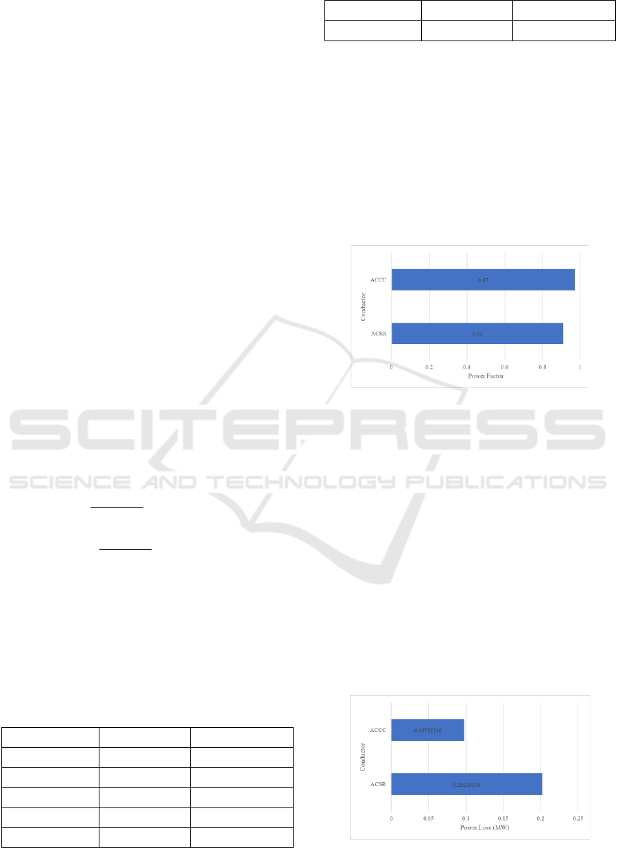
Table 3: Summary of calculations.
ACSR
ACCC
Power Factor
0.91
0.97
85.8105
100.7348
0.1966
0.0947
0.00558
0.00287
0.20218
0.0976
87
100.8323
87.845
99.9
Starting first with the power factor, the
calculations for the power factor of ACSR resulted in
0.91. Power factor has a range of 0 to 1 with 0 being
very inefficient and 1 being very efficient and
therefore less power being wasted (Dani &
Hasanuddin, 2018). 0.91 or 91% for power factor is
already a good indication of efficiency, but it can still
be improved since the upper limit is 1 or 100%. After
the reconfiguration process into ACCC conductor, the
power factor increased to 0.97 or 97% which is a
6.59% improvement.
Figure 9: Comparison of power factor.
That number may sound insignificant, but if seen
in the long term, such as in a few months or years,
6.59% will save electricity costs significantly. 6.59%
in substation value can also be used to power several
houses.
Moving on to the next variable which is power
loss. The total power losses are shown as
and
for both ACSR and
ACCC conductor respectively. Before the
reconfiguration process, the total power loss is 0.2022
MW which is significantly more than after the
reconfiguration process which is only 0.0976 MW.
This equates to around 51.75% decrease of power loss
which is very significant and in the long run will save
even more power and benefit everyone economically.
The figure below shows the comparison between both
power losses.
Figure 10: Comparison of total power loss.
Increasing the Efficiency of Bolangi Substation Extension by Using ACCC Conductor on 150 KV Sungguminasa-Bolangi Overhead Power
Line
471

By dividing the corona losses by the total power
losses, we can see that corona losses only contribute
about 2.76 – 2.94% of the total power losses.
The last variable that’s compared is the
transmission efficiency which is defined as the ratio
between the power and the total power, the latter of
which includes the total power losses and the power
combined. Before the reconfiguration process, ACSR
conductor has a transmission efficiency of 97.845%.
After reconfiguring into ACCC, we have a
transmission efficiency of 99.9%. Comparing these
two values, there’s an increase of around 2.1% in
transmission efficiency. Similar to power factor, the
effect of this will be more significant as time goes on.
Figure 11: Comparison of transmission efficiency.
5 CONCLUSIONS
Based on this research which carries out the process
of reconfiguring the conductor on High Voltage
Overhead Lines from ACSR to ACCC conductor,
there are several conclusions that can be drawn.
1. The reconfiguration process from ACSR to
ACCC resulted in the increase of power
factor by 6.59% from 0.91 to 0.97.
2. The reconfiguration process from ACSR to
ACCC resulted in the decrease of power loss
by 51.75% from 0.2022 MW to 0.09756
MW.
3. The reconfiguration process from ACSR to
ACCC resulted in the increase of
transmission efficiency by 2.1% from
97.845% to 99.9%.
4. Other factors such as air density,
temperature, and atmospheric conditions
only contribute around 2.76 – 2.94% to the
total power loss of the system.
REFERENCES
Arismunandar, A., & Kuwahara, S. (2004). Buku Pegangan
Teknik Tenaga Listrik Jilid II Saluran Transmisi (2nd
ed.). PT. Pradnya Paramita.
Bryant, D. (2019). Engineering Transmission Lines with
High Capacity Low Sag ACCC® Conductors. Capacity
| CTC ACCC Conductor.
Chen, G., Wang, X., Wang, J., Liu, J., Zhang, T., & Tang,
W. (2012). Damage investigation of the aged
aluminium cable steel reinforced (ACSR) conductors in
a high-voltage transmission line. Engineering Failure
Analysis, 19, 13–21.
https://doi.org/10.1016/j.engfailanal.2011.09.002
Dani, A., & Hasanuddin, M. (2018). Perbaikan Faktor Daya
Menggunakan Kapasitor Sebagai Kompensator Daya
Reaktif (Studi Kasus STT Sinar Husni). STMIK Royal
– AMIK Royal, 1(1), 673–678.
F. W. Peek. (1929). Dielectric phenomena in high-voltage
engineering (3rd ed.). New York McGraw-Hill Book
Company, Inc.
Handayani, O., Darmana, T., & Widyastuti, C. (2019).
Analisis Perbandingan Efisiensi Penyaluran Listrik
Antara Penghantar ACSR dan ACCC pada Sistem
Transmisi 150kV. Energi & Kelistrikan, 11(1), 37–45.
https://doi.org/10.33322/energi.v11i1.480
Imam G. (2017). Analisa Rugi Penghantar Rekonduktoring
Acsr – Accc Saluran Udara Tegangan Tinggi 150 Kv
Mranggen Incomer. TJ Mechanical Engineering and
Machinery.
Kenge, A. v., Dusane, S. v., & Sarkar, J. (2016). Statistical
analysis & comparison of HTLS conductor with
conventional ACSR conductor. 2016 International
Conference on Electrical, Electronics, and
Optimization Techniques (ICEEOT), 2955–2959.
https://doi.org/10.1109/ICEEOT.2016.7755241
Lalonde, S., Guilbault, R., & Langlois, S. (2018).
Numerical Analysis of ACSR Conductor–Clamp
Systems Undergoing Wind-Induced Cyclic Loads.
IEEE Transactions on Power Delivery, 33(4), 1518–
1526. https://doi.org/10.1109/TPWRD.2017.2704934
Qiao, K., Zhu, A., Wang, B., Di, C., Yu, J., & Zhu, B.
(2020). Characteristics of Heat Resistant Aluminum
Alloy Composite Core Conductor Used in overhead
Power Transmission Lines. Materials, 13(7), 1592.
https://doi.org/10.3390/ma13071592
Slegers, J. (2011). Transmission Line Loading: Sag
Calculations and High-Temperature Conductor
Technologies.
W. S. Peterson. (1933). Development of a Corona Loss
Formula.
Wareing, B. (2018). Types and Uses of High Temperature
Conductors.
Wustqa, D. U., Listyani, E., Subekti, R., Kusumawati, R.,
Susanti, M., & Kismiantini, K. (2018). Analisis Data
Multivariat Dengan Program R. Jurnal Pengabdian
Masyarakat MIPA Dan Pendidikan MIPA, 2(2), 83–86.
https://doi.org/10.21831/jpmmp.v2i2.21913.
iCAST-ES 2022 - International Conference on Applied Science and Technology on Engineering Science
472
