Computer Modeling of the Equilibrium Position Magnetization

Precession in the Ferrite Plate

V. S. Vlasov

, D. A. Suslov

, V. G. Shavrov

and V. I. Shcheglov

Syktyvkar State University, Syktyvkar, Russia

Kotel’nikov Institute of Radio Engineering and Electronics, Russian Academy of Sciences, Moscow, Russia

Keywords: Nonlinear Magnetization Precession, Computer Modelling, Ferrite Plate.

Abstract: Nonlinear equilibrium position magnetization precession in a normally magnetized ferrite plate is modeled in

the Matlab system. The magnetization motion equations for 3 cases are given: the isotropic plate, the plate

with uniaxial anisotropy and the plate with cubic anisotropy. Differential equation system for magnetization

vector relative to magnetization components is solved by Runge-Kutta method in the Matlab. The code of the

program for modeling the magnetization dynamics is given. The program allows to build parametric portraits

of the magnetization and study their features under various types of the plate anisotropy. The features of

parametric portraits for these three cases of the anisotropy are considered.

1 INTRODUCTION

There is the great interest in modeling the dynamics

of nonlinear magnetic systems (Vlasov et al., 2022;

Vlasov et al., 2020). It is caused by promising

applications of magnetic nanostructures in

spintronics and nanoelectronics (Shelukhin et al.,

2022; Barman et al., 2020). Computer modeling is

also relevant due to the impossibility of analytical

solution of the magnetization dynamics nonlinear

problems (Shavrov and Shcheglov, 2021). One of the

interesting types of the magnetization vector

precession in planar structures is the equilibrium

position precession. Such precession can be observed

in the perpendicular magnetized plate (Shavrov and

Shcheglov, 2021). In this case, the DC field is smaller

than the demagnetization field and the magnetization

vector is deviated from the direction of the field in the

equilibrium state. When the alternating field is turned

on, the precession of the magnetization vector

appears relative to the equilibrium position.

Moreover, the equilibrium position moves along the

"big circle" of the precession portrait and we see the

rings filled the "big circle". So, the realization of

"precession in precession" is obtained (Shavrov and

Shcheglov, 2021; Vlasov et al., 2011).

https://orcid.org/0000-0001-6902-608X

https://orcid.org/0000-0002-1962-1195

https://orcid.org/0000-0003-0873-081X

The magnetization dynamics for the equilibrium

position precession cannot be found by using

analytical formulas. Therefore, the only theoretical

way to study the equilibrium position precession is

the computer modeling using numerical solution

methods (Shavrov and Shcheglov, 2021; Vlasov et

al., 2012; Vlasov et al., 2013). Matlab package

solution methods are used to simulate the motion of

the magnetization vector in the present paper.

The paper is devoted to modeling the equilibrium

position precession with the symmetric and

asymmetric DC fields orientation in the isotropic

ferrite plate and for cases of the uniaxial and cubic

anisotropy (Shavrov and Shcheglov, 2021).

2 GEOMETRY AND BASIC

EQUATIONS

2.1 Geometry of the Problem

Let’s consider the normally magnetized ferrite plate.

The 3 cases of equilibrium position precession for

different types of the plate anisotropy are studied: 1.

the isotropic plate; 2. the plate with uniaxial

Vlasov, V., Suslov, D., Shavrov, V. and Shcheglov, V.

Computer Modeling of the Equilibrium Position Magnetization Precession in the Ferrite Plate.

DOI: 10.5220/0011906700003612

In Proceedings of the 3rd International Symposium on Automation, Information and Computing (ISAIC 2022), pages 115-120

ISBN: 978-989-758-622-4; ISSN: 2975-9463

 2023 by SCITEPRESS – Science and Technology Publications, Lda. Under CC license (CC BY-NC-ND 4.0)

115

anisotropy; 3. the plate with cubic magnetic

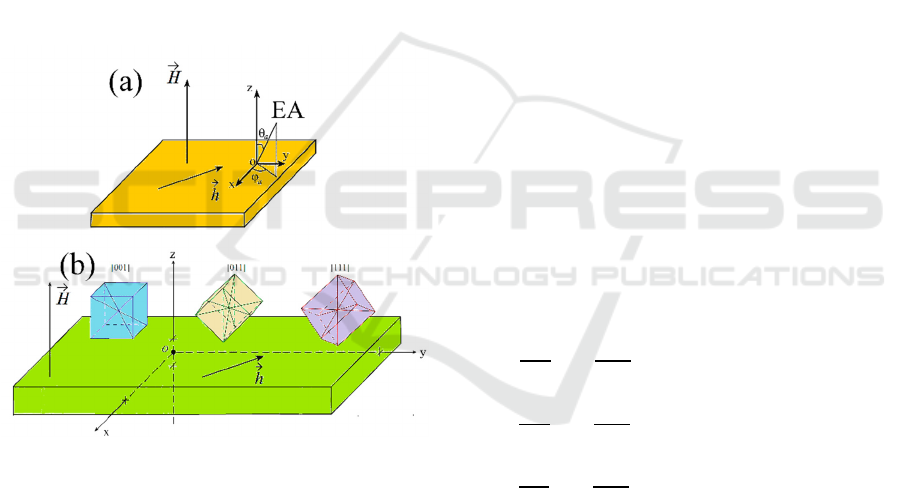
anisotropy. The general geometry of the problem is

illustrated in Figure 1. Figure 1a shows the plate with

uniaxial anisotropy. Figure 1b illustrates the plate

with cubic anisotropy. The ferrite plate is magnetized

by the DC field perpendicular to its plane, the

alternating field is applied in the plane of the plate.

The xOy plane of the Cartesian coordinate system

Oxyz coincides with the plane of the plate. The z axis

is perpendicular to the plate plane. For the case of the

isotropic ferrite plate, the DC field may also have

weak components in the plane of the plate.

Firstly, let us consider in detail the geometry of

the problem for the ferrite plate with uniaxial

magnetic anisotropy (Shavrov and Shcheglov, 2021).

The easy axis (EA) is deviated from the normal to the

plate plane by the arbitrary angle. Such geometry of

the problem is shown in Figure 1a. The direction of

the EA is given by 2 angles in the spherical coordinate

system 𝜃



, 𝜑



Figure 1. Geometry of the problem.

For the case of the plate with cubic anisotropy,

three variants of the orientation of the cubic

crystallographic cell are considered in Figure 1b:

1) ORIENTATION [001]: one of the crystallographic

axes of the type [001] which is the edge of the cube is

directed along the normal from the plate plane;

2) ORIENTATION [011]: one of the axes of the type

[011] is directed along the normal from the plate

plane, i.e. the diagonal of the cube face;

3) ORIENTATION [111]: one of the axes of type

[111], i.e. the spatial diagonal of the cube, is directed

along the normal from the plane of the plate (Vlasov

et al., 2013).

2.2 Basic Equations

The problem of the magnetization vector dynamic

behavior is solved in the coordinate system associated

with the DC field, i.e. Oxyz. The expressions for the

energy and the uniaxial anisotropy field for the case

of the easy axis rotated by angles 𝜃



, 𝜑



are obtained

in the work (Shavrov and Shcheglov, 2021). The

expressions for the energy and fields of the cubic

anisotropy, for orientations [001], [011], [111] are

obtained similarly in work (Vlasov et al., 2013).

We further assume that the DC field 𝐻



⃗

is not

sufficient to align the magnetization vector in the

equilibrium state perpendicular to the plane of the

plate. The components of the alternating field have

the form:

ℎ



=ℎ



𝑠𝑖𝑛

(

2𝜋𝐹𝑡

)

, ℎ



=−ℎ



𝑐𝑜𝑠

(

2𝜋𝐹𝑡

)

(1)

where F – the alternating field frequency, h

– its

amplitude.

The magnetization equilibrium position

precession is possible to observe for such magnetic

fields orientation relative to the plate plane, in certain

circumstances. This precession type is the

equilibrium position motion around the direction of

the DC field with the frequency significantly lower

than alternating field frequency.

To solve the problem of the magnetization vector

dynamic behavior we use the Landau–Lifshitz

magnetization motion equations with the dissipative

Gilbert term (LLG) (Shavrov and Shcheglov, 2021):







=−







𝑚



+𝛼𝑚



𝑚



𝐻



−𝑚



−

𝛼𝑚



𝑚



𝐻



−𝛼𝑚





+𝑚





𝐻



 , (2)







=−







𝑚



+𝛼𝑚



𝑚



𝐻



−𝑚



−

𝛼𝑚



𝑚



𝐻



−𝛼

(

𝑚





+𝑚





)

𝐻



, (3)







=−







𝑚



+𝛼𝑚



𝑚



𝐻



−𝑚



−

𝛼𝑚



𝑚



𝐻



−𝛼𝑚





+𝑚





𝐻



, (4)

where 𝑚



⃗

=𝑀



⃗

𝑀



 – the normalized magnetization

vector, 𝑚



– its components in the Cartesian

coordinate system, 𝑀



– the saturation

magnetization, 𝛾 –the gyromagnetic ratio (𝛾 > 0), 𝛼 –

magnetic dissipation parameter, 𝐻



– the

components of the effective field. In the case of the

isotropic plate, the components of the effective field

included in equations (2-4) have the form:

𝐻



=ℎ



+𝐻



, (5)

𝐻



=ℎ



+𝐻



, (6)

ISAIC 2022 - International Symposium on Automation, Information and Computing

116

𝐻



=𝐻



−4𝜋𝑀



𝑚



. (7)

For the cases of the plate with uniaxial and cubic

anisotropy, the components of effective fields have

the following form:

𝐻



=ℎ



+𝐻



+𝐻



, (8)

𝐻



=ℎ



+𝐻



+𝐻



, (9)

𝐻



=𝐻



−4𝜋𝑀



𝑚



+𝐻



. (10)

Let's look at the components of the anisotropy

field included in expressions (8-10). For the case of

uniaxial anisotropy with angles 𝜃



, 𝜑



the

expressions for the anisotropy field components have

following form (Shavrov and Shcheglov, 2021):

𝐻



=𝐻









(−𝑚



(

𝑐𝑜𝑠



𝜃



𝑐𝑜𝑠



𝜑



𝑠𝑖𝑛



𝜑



)

+𝑚



𝑠𝑖𝑛



𝜃



𝑠𝑖𝑛𝜑



𝑐𝑜𝑠𝜑



𝑚



𝑠𝑖𝑛𝜃



𝑐𝑜𝑠𝜃



𝑐𝑜𝑠𝜑



, (11)

𝐻



=𝐻









(𝑚



𝑠𝑖𝑛



𝜃



𝑠𝑖𝑛𝜑



𝑐𝑜𝑠𝜑



−

𝑚



(

𝑐𝑜𝑠



𝜃



𝑠𝑖𝑛



𝜑



+𝑐𝑜𝑠



𝜑



)

𝑚



𝑠𝑖𝑛𝜃



𝑐𝑜𝑠𝜃



𝑠𝑖𝑛𝜑



, (12)

𝐻



=𝐻









(𝑚



𝑠𝑖𝑛𝜃



𝑐𝑜𝑠𝜃



𝑐𝑜𝑠𝜑



𝑚



𝑠𝑖𝑛𝜃



𝑐𝑜𝑠𝜃



𝑠𝑖𝑛𝜑



−𝑚



𝑠𝑖𝑛



𝜃



), (13)

where 𝐾 – the uniaxial anisotropy constant.

In the case of the cubic anisotropy and the

orientation [001], the components of the anisotropy

field can be written as follows:

𝐻



=𝐻



()









𝑚



(𝑚





+𝑚





), (14)

𝐻



=𝐻



()









𝑚



(𝑚





+𝑚





), (15)

𝐻



=𝐻



()









𝑚



(𝑚





+𝑚





). (16)

In the case of cubic anisotropy and orientation [001],

the components of the anisotropy field have the

following form:

𝐻



=𝐻



()









𝑚



(𝑚





+𝑚





), (17)

𝐻



=𝐻



()









𝑚



(2𝑚





+𝑚





−𝑚





), (18)

𝐻



=𝐻



()









𝑚



(2𝑚





−𝑚





+𝑚





). (19)

The cubic anisotropy fields for orientation [111] look

like this:

𝐻



=𝐻



()









(𝑚





+𝑚



𝑚





−

√

2𝑚





𝑚



√

𝑚





𝑚



), (20)

𝐻



=𝐻



()









(𝑚





+𝑚





𝑚



√

𝑚



𝑚



𝑚



), (21)

𝐻



=𝐻



(



)









(





𝑚





−

√





𝑚





√

2𝑚



𝑚





). (22)

where 𝐾



– the first constant of cubic anisotropy.

3 SOLUTION ALGORITHM

Let's consider the algorithm for solving the problem

in the Matlab system. The LLG equations system (2-

4) is solved by the 4-5 orders Runge-Kutta method

into the Matlab package with the accuracy control at

each step. Firstly, parameters are entered in the task.

The right part of the LLG equations system is

designed as the separate function. Next, the numerical

solution of the system is implemented. The results of

the numerical solution are output in the magnetization

precession portraits graphs form m

), which are

projections of the magnetization phase trajectories.

The content of the main program for the Matlab is

shown in Listing 1.

Listing 1: The listing of the main program.

close all

clear all

global alf h F1 Hx Hy H0 M0 Ku teta_a

fi_a K1

neq=3;

M0=280/(4*pi);

gamma=1.756e7;

H0=252;

alf=0.3;

h=3;

F1=1e8/(gamma*M0);

Hx=0.1*0;

Hy=0;

Ku=0;

teta_a=10*pi/180;

fi_a=0;

K1=8;

for i=1:neq

abt(i)=5e-6;

end;

teta0=acos(H0/(4*pi*M0));

ink(1)=sin(teta0);

ink(2)=0;

ink(3)=cos(teta0);

tras=1000;

Computer Modeling of the Equilibrium Position Magnetization Precession in the Ferrite Plate

117

options = odeset('RelTol',5e-

6,'AbsTol',abt);

[T,Y] = ode45(@y_m2022_2,[0

tras],ink,options);

Nt=length(T);

T1=T(round(Nt/2):Nt);

mx1=Y(round(Nt/2):Nt,1);

my1=Y(round(Nt/2):Nt,2);

figure(1)

plot(mx1,my1,'LineWidth', 2);

set(gca,'FontSize',36,'LineWidth', 4);

xlabel('m_x','FontSize',48);

ylabel('m_y','FontSize',48);

Let's describe the text of the main program. First

of all, the global parameters are set. The

alf – the

magnetic dissipation parameter,

h – the alternating

field amplitude,

F1 – the alternating field frequency,

Hx, Hy – components of the weak DC field applied

in the plate plane, H0 – the main DC magnetizing

field applied along the normal from the plate plane,

M0 – the saturation magnetization of the plate,

Ku –

the uniaxial anisotropy constant, teta_a, fi_a –

angles 𝜃



, 𝜑



, K1 – the first constant of the cubic

anisotropy.

Next, the program introduces the

parameter

neq=3 corresponding to the number of

differential equations in the system and the values of

the listed system parameters. The absolute accuracy

is introduced in the for loop for the 3 components of

magnetization corresponding to the variables

abt(i)=5e-6 for the system of differential

equations LLG solution.

teta0 is the deviation angle

of the magnetization from the normal to the plate

plane, which is calculated by the formula taken from

work (Vlasov et al., 2011). The initial values of the

unit magnetization vector components

ink(1),

ink(2), ink(3) are calculated by using this angle.

tras=1000 is the final time for the dynamics of

magnetization calculation (in relative units). The set

of parameters

options gives the relative and

absolute accuracy of the solution of the LLG system.

The

ode45 function implements the solution of the

LLG system by the Runge-Kutta 4-5 orders method.

After the numerical solution of the LLG equations

system, the arrays

mx1, my1 are determined in the

program. The steady-state values of the

magnetization components 𝑚



, 𝑚



are written in the

arrays. The

plot function implements the plotting of

the magnetization precession portrait.

The right part of the differential equations system

is described as the separate function in the Matlab

system. 2 different functions are introduced to

describe the right side of the LLG system for all three

cases of the anisotropy. The function corresponding

the LLG system for the case of the isotropic plate and

the case of uniaxial anisotropy (case 1) is shown in

Listing 2.

Listing 2: The LLG system function. Case 1.

function f=y_m2022_1(t,m)

global alf h F1 Hx Hy H0 M0 Ku teta_a

fi_a K1

cg=-1/(1+alf*alf);

neq=3;

f=zeros(neq,1);

mx=m(1);

my=m(2);

mz=m(3);

Heu_x=2*Ku/M0*(-

mx*(cos(teta_a)^2*cos(fi_a)^2+sin(fi_a)

^2)+...

my*sin(teta_a)^2*sin(fi_a)*cos(fi_a)+

mz*sin(teta_a)*cos(teta_a)*cos(fi_a));

Heu_y=2*Ku/M0*(mx*sin(teta_a)^2*sin(fi_

a)*cos(fi_a)-...

my*(cos(teta_a)^2*sin(fi_a)^2+cos(fi_a)

^2)+mz*sin(teta_a)*cos(teta_a)*sin(fi_a

));

Heu_z=2*Ku/M0*(mx*sin(teta_a)*cos(teta_

a)*cos(fi_a)+...

my*sin(teta_a)*cos(teta_a)*sin(fi_a)-

mz*sin(teta_a)^2);

hx=(h*sin(2*pi*F1*t)+Hx+Heu_x)/M0;

hy=(-h*cos(2*pi*F1*t)+Hy+Heu_y)/M0;

hz=(H0-4*pi*mz*M0+Heu_z)/M0;

fx=my*hz-mz*hy;

fy=mz*hx-mx*hz;

fz=mx*hy-my*hx;

fhx=my*fz-mz*fy;

fhy=mz*fx-mx*fz;

fhz=mx*fy-my*fx;

f(1)=cg*(fx + alf*fhx);

f(2) = cg*(fy + alf*fhy);

f(3)= cg*(fz + alf*fhz);

end

The function implements the assignment of the right

side of the LLG system (2-4) in the case of the

isotropic plate or the uniaxial anisotropy. Moreover,

the solution of the system is carried out in relative

units: time is normalized by the value 1(𝛾𝑀



)

⁄

, the

alternating field frequency is normalized by the value

𝛾𝑀



(in the main program).

ISAIC 2022 - International Symposium on Automation, Information and Computing

118

The function of the LLG system for the case of the

cubic anisotropy plate (case 2) is given in Listing 3.

Listing 3: The LLG system function. Case 2.

function f=y_m2022_2(t,m)

…

a_orient = '111';

switch a_orient

case '001'

Ha_x=2*K1/M0*mx*(my^2+mz^2);

Ha_y=2*K1/M0*my*(mz^2+mx^2);

Ha_z=2*K1/M0*mz*(mx^2+my^2);

case '011'

Ha_x=2*K1/M0*mx*(my^2+mz^2);

Ha_y=2*K1/M0*my*(2*mx^2+my^2-

mz^2);

Ha_z=2*K1/M0*mz*(2*mx^2-

my^2+mz^2);

case '111'

Ha_x=2*K1/M0*(mx^3+mx*my^2-

sqrt(2)*mx^2*mz+sqrt(2)*my^2*mz);

Ha_y=2*K1/M0*(my^3+mx^2*my+2*sqrt(2)*mx

*my*mz);

Ha_z=2*K1/M0*(4/3*mz^3-

sqrt(2)/3*mx^3+sqrt(2)*mx*my^2);

end

hx=(h*sin(2*pi*F1*t)+Hx+Ha_x)/M0;

hy=(-h*cos(2*pi*F1*t)+Hy+Ha_y)/M0;

hz=(H0-4*pi*mz*M0+Ha_z)/M0;

…

The listing is given from the end of the line mz=m(3)

to the definition of the variable fx. The fragments of

the

function y_m2022_2(t,m) before the end of

the line

mz=m(3) and after determining the variable

fx, completely repeat the listing of the previous

function

function y_m2022_1(t,m). To separate

the different cases of orientation of the

crystallographic cell the text variable

a_orient is

introduced, for which one of 3 values must be set:

'001', '011', '111'.

4 RESULTS OF NUMERICAL

SOLUTION OF THE LLG

SYSTEM

Let's have a look at the main results of the numerical

solution of the LLG system obtained using the

described calculation program. The plots of all 3

cases of the solution (1. Isotropic plate; 2. Plate with

uniaxial anisotropy; 3. Plate with cubic anisotropy)

are shown in Figure 2. The values of the parameters

given in Listing 1 are used for constructing

calculations Figure 2. The parameters are given in the

CGS system of units. The frequency of the alternating

field is F=100 MHz and corresponds to the variable

F1. This value is divided by the value gamma*M0 due

to the transition to the relative times and frequencies

in the program text.

Let's consider the features of precession portraits

in Figure 2. In the case of the symmetric DC field and

the isotropic plate, small rings uniformly fill the

precession portrait along the generatrix of the large

circle. Such precessional portrait is shown in Figure

2a. The presence of the rings accumulations and

sparsities on the precessional portrait is visible in the

other sub-drawings. The mechanism of formation of

the ring accumulations and sparsities was described

in works (Shavrov and Shcheglov, 2021; Vlasov et

al., 2011; Vlasov et al., 2012; Vlasov et al., 2013) on

the basis of energy and vector models.

Figure 2: Precession portraits of magnetization for different

cases of the anisotropy: (a) the isotropic plate with the

symmetric DC field; (b) the isotropic plate with the weak

asymmetric field applied along x-axis; (c) the case of the

uniaxial anisotropy; (d) the cubic anisotropy with the

orientation [001]; (e) the cubic anisotropy with the

orientation [011]; (f) the cubic anisotropy with the

orientation [111].

The ring accumulations occur at the angle of 90

degrees to the weak DC field applied in the plane for

the isotropic plate. The such case is shown in Figure

2b. The additional weak DC field is directed along the

x axis and equal to 𝐻



=0.1 Oe. Therefore, the rings

Computer Modeling of the Equilibrium Position Magnetization Precession in the Ferrite Plate

119

accumulation in this portrait is located at the angle of

90 degrees with respect to the x axis and

counterclockwise rotated. The polar and azimuthal

angles that correspond to the orientation of the easy

axis are 𝜃



= 10°, 𝜑



=0 for the case of uniaxial

anisotropy (Figure 2c). Thus the projection of the

anisotropy axis onto the plate plane is parallel to the

x coordinate axis. The axis is 10° angle with the

normal from the plate. The similar rings

accumulations and sparsities are observed in Figure

2c, as in the case of the asymmetric DC field (Figure

2b) directed along the x axis. The number of ring

accumulations and sparsities depends on the number

of minima and maxima of the anisotropy energy in

the projection onto the plate plane for the case of

cubic anisotropy (Figure 2d, e, f). Figure 2d is

constructed for orientation [001]. The value of the

cubic anisotropy constant is 𝐾



=160 erg/cm

. 4 ring

accumulations are visible in Figure 2d. The

accumulations correspond to the presence of 4

minima and maxima along the precession forming the

large circle. Figure 2e is constructed for orientation

[011]. The value of the cubic anisotropy constant is

𝐾



=5 erg/cm

. 2 ring accumulations are visible in Fig.

2e corresponding to 2 minima and maxima along the

generatrix of the large circle. Figure 2f is constructed

for orientation [111]. The value of the cubic

anisotropy constant 𝐾



=8 erg/cm

. 3 thickenings are

visible in Figure 2f, corresponding to 3 minima and

maxima along the generatrix of the large circle.

5 CONCLUSIONS

The calculation computer program has been

developed in the Matlab system. The computer

simulation of the equilibrium position precession in

the ferrite plate has been carried out in 3 cases. The

first case is the isotropic plate, the second case is the

plate with uniaxial anisotropy, the third case is the

plate with cubic anisotropy. The listing of the

calculation program text is given. The program

consists of the main module and two auxiliary

functions to describe the right-hand side of the

Landau-Lifshitz-Gilbert system of differential

equations. The explanations for the features of the

obtained magnetization precession portraits based on

the presence of maxima and minima of anisotropy

energy along the large precession circle are given.

ACKNOWLEDGEMENTS

This work has been supported by the Russian Science

Foundation, project no. 21-72-20048.

REFERENCES

Vlasov, V. S., Makarov, P. A., Shavrov, V. G. and

Shcheglov, V. I. (2022). Impact excitation of magnetic

oscillations by an elastic displacement pulse. Journal of

Communications Technology and Electronics, 67(7):

876–881.

Vlasov, V. S., Lomonosov, A. M., Golov, A. V., Kotov, L.

N., Besse, V., Alekhin, A., Kuzmin, D. A., Bychkov, I.

V. and Temnov, V. V. (2020). Magnetization switching

in bistable nanomagnets by picosecond pulses of

surface acoustic waves. Phys. Rev. B, 101(2): 024425.

Shelukhin, L. A., Gareev, R. R., Zbarsky, V., Walowski, J.,

Münzenberg, M., Pertsev, N. A. and Kalashnikova, A.

M. (2022). Spin reorientation transition in

CoFeB/MgO/CoFeB tunnel junction enabled by

ultrafast laser-induced suppression of perpendicular

magnetic anisotropy. Nanoscale, 14: 8153-8162.

Barman, A., Mondal, S., Sahoo, S. and De, A. (2020).

Magnetization dynamics of nanoscale magnetic

materials: a perspective. J. Appl. Phys. 128: 170901.

Shavrov, V. G. and Shcheglov, V. I. (2021). Ferromagnetic

resonance in orientational transition conditions, CRC

Press. Boca Raton, 1

edition.

Vlasov, V. S., Kotov, L. N., Shavrov, V. G., and Shcheglov,

V. I. (2011). Forced nonlinear precession of the

magnetization vector under the conditions of an

orientation transition. Journal of Communications

Technology and Electronics, 56(1): 73–84.

Vlasov, V. S., Kotov, L. N., Shavrov, V. G., and Shcheglov,

V. I. (2012). Asymmetric excitation of the two-order

magnetization precession under orientational transition

conditions. Journal of Communications Technology

and Electronics, 57(5): 453–467.

Vlasov, V. S., Kirushev, M. S., Kotov, L. N., Shavrov, V.

G., and Shcheglov, V. I. (2013). The second-order

magnetization precession in an anisotropic medium.

Part 2: The cubic anisotropy. Journal of

Communications Technology and Electronics, 58(9):

847–862.

ISAIC 2022 - International Symposium on Automation, Information and Computing

120