Depth Map Estimation of Focus Objects Using Vision Transformer

Chae-rim Park

, Kwang-il Lee

and Seok-je Cho

Control and Automation Engineering, Korea Maritime and Ocean University, Korea

Keywords: Computer Vision, Object Detection, Transformer, Attention, ViT.

Abstract: Estimating Depth map from image is critical in a variety of tasks such as 3D object detection and extraction.

In particular, it is an essential task for Robot, AR/VR, Drone, and Autonomous vehicles, and plays an

important role in Computer vision. In general, stereo technique is used to extract the Depth map. It matches

two images a different locations in the same scene and determines and output the distance according to the

size of the relative motion. In this paper, I propose a method for extracting Depth map using vision

Transformer(ViT) through input images from various environments. After automatically focusing on the

object in the image using ViT, semantic segmentation is performers to Computer vision, and fine-tuning

images with fewer resources represents a better Depth map.

1 INTRODUCTION

Depth map provides information related to the

distance from a fixed point in time to the surface of a

subject in an image containing a two-dimensional

object. The 3D object information obtained through

Depth map is useful in 3D modeling, and it can be

inferred that obscuring between objects is potentially

occurring. A representative method of outputting

such a Depth map is a stereo matching technique. It is

designed to obtain the matching values of two images

taken from different locations in the same scene first,

and to determine the distance according to the relative

motion size for the same matching value. That is, it

can be seen that it relies on images obtained with the

left and right eyes of the person.

In addition to the stereo matching technique,

studies to predict the depth of the image have been

steadily conducted. The first LiDAR is a technology

that can collect physical properties, distances to

objects, or 3D image information by illuminating a

laser beam on a target. Original LiDAR had

limitations due to a low sampling rate, But in 2020,

Researchers at Stanford University overcame these

limitations and demonstrated the completion of the

Depth map. Next, DenseDepth with an encoder-

decoder structure is a convolutional neural network

that outputs a high-resolution Depth map from a

https://orcid.org/0000-0001-9985-3967

https://orcid.org/0000-0002-8307-9003

https://orcid.org/0000-0001-9979-2252

single image through transmission learning. This

results in a high-quality Depth map representing more

accurate and detailed boundaries using augmented

learning strategies and pre-trained high-performance

networks.

In this study, the Depth map is generated using a

new network, Vision Transformer(ViT). It proposes a

technique that automatically focuses by exploring 3D

objects in images and measures and extracts accurate

Depth maps. The image is calibrated using the

Retinex algorithm when the image enters the input,

and then the image is separated by measuring weights

between separated patches and reconstructed based

on them. The extracted image enters the input of the

ViT encoder and generates an excellent Depth map

through the proposed network. ViT complements the

self-Attention elements that were restricted in the

field of vision, and shows far superior results to the

conventional Convolution Neural Network(CNN)

structures. The backpropagated image is put into the

input of the ViT encoder and a final Depth map is

generated through various processes.

150

Park, C., Lee, K. and Cho, S.

Depth Map Estimation of Focus Objects Using Vision Transformer.

DOI: 10.5220/0011908700003612

In Proceedings of the 3rd International Symposium on Automation, Information and Computing (ISAIC 2022), pages 150-155

ISBN: 978-989-758-622-4; ISSN: 2975-9463

 2023 by SCITEPRESS – Science and Technology Publications, Lda. Under CC license (CC BY-NC-ND 4.0)

2 ENHANCEMENT OF OBJECT

DEBLURRING IN IMAGES

Image correction is basically required in order to

obtain a Depth map in various environments. After

correcting the input image using Retinex, the loss

value between the resulting image and the predicted

image is measured through a newly designed

encoder-decoder architecture and backpropagated

through Improver.

2.1 Retinex

Most images exhibit a mixture of areas with high

brightness by light and areas with darkened shadows

due to limited brightness, resulting in a poor object

recognition. The process of improving the contrast of

the image is performed before the image enters the

input of the architecture. It is the role of the Retinex

algorithm to reduce illumination light sources and

calibrate images with reflective components based on

human visual models.

Experiments by Land et al. have demonstrated that

the color of an object perceived by a human visual

organ can be expressed as a product of the light source

and the reflective components of the object as shown

in Equation (1). In addition, Weber-Fechner’s law is

applied that human visual perception has a log

relationship between the actual applied stimulus

value and the perceived sense. If the reflective

component of Equation (1) is mainly expressed, it can

be expressed as Equation (2).

𝐼=𝑅∙ 𝐿 (1)

𝑅=𝑙𝑜𝑔









(2)

𝑅=𝑙𝑜𝑔



𝐼



−𝑙𝑜𝑔



𝐹∗𝐼



(3)

In term of the formula, brightness image I is the

product of the two components, illumination

component L and reflectance component R. The

above equation means that the lighting component

can be estimated and the index reflection component

unique to the object may be determined through an

arithmetic method. The subtraction law of log in

Equation (2) and the peripheral function are

expressed as Equation (3). Here, F is used to estimate

the lighting component of the surrounding area, and a

Gaussian filter or an average filter is mainly used to

estimate the lighting component.

2.2 Image Feature Extraction

In this paper, the proposed architecture extracts

features in patch units when images are input,

measures weights, separates them, and then

reconstructs them, which are scaled to a stack form.

To reconstruct the feature map, it proposeds a new

architecture by introducing the Nested module into

the architecture proposed by G. Hongyon et al. The

overlay module outputs object detection, image

deblurring, and high-resolution images using two or

more convolution layers to produce excellent results.

It can also improve the flow of information and

efficiently handle the slope loss problem of the

network. The newly proposed architecture optimizes

complexly represented images more efficiently and

easily models them to capture the details of the

images.

Figure 1(a)(light blue block) is a Retinex algorithm

process. By separating the lighting component and

the reflective component of the input image, the

image is corrected by reducing the ratio of the lighting

component and increasing the ratio of the reflective

component. Figure 1(b)(light purple block) shows

multiple overlapping encoder-decoders with the

proposed architecture.

2.3 Improver

The error value between the resulting image extracted

through the architecture and the predicted image is

obtained and backpropagated through the Improver.

Improver is a multi-perceptron structure that plays a

central role in performance improvement for

extracted images. It reduces errors present by

backpropagation algorithms that update weights from

behind to back. The Improver architecture includes

input, hidden, and output layers, which shares all the

weight values because the relationship between them

is completely connected. Quantitatively calculation

how much the loss value occurring between them

affects and then backpropagates again. The error

between the two uses the Mean Square Error. This is

a measure used to when dealing with the difference

between the estimated value or the value predicted by

the model and the value observed in the real

environment, and measures the difference in pixel

values between each image.

𝑀𝑆𝐸 =





𝛴



𝑂−𝐺





(4)

In Equation (4), n is the size, O is the extracted

image, and G is the predicted image. The

backpropagation is performed after determining the

loss value between the extracted image and the

predicted image using the Improver. Since this

process is performed on a patch-by-patch basis,

parameters are relatively reduced and rapid results

can be derived and feedback can be provided.

Depth Map Estimation of Focus Objects Using Vision Transformer

151

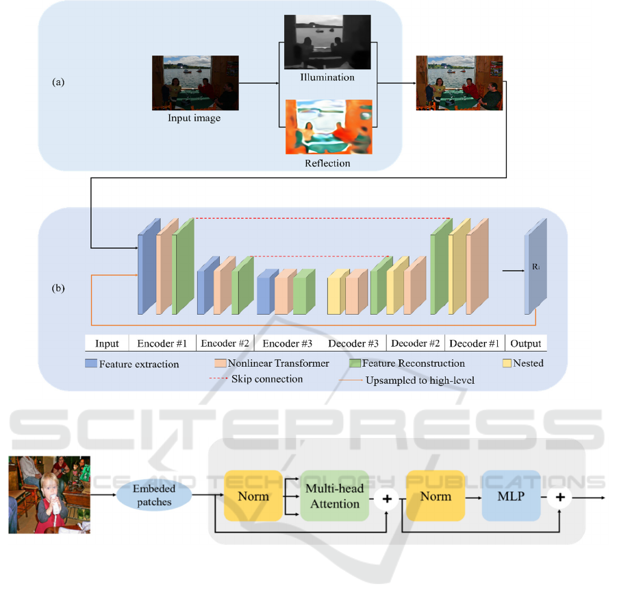
Figure 1: Proposed Architecture.

Figure 2: Transformer Encoder in Vision Transformer.

3 VISION TRANSFORMER

A Vision Transformer (ViT) is a converter that

processes images. Google Research’s brain team was

born with the idea of processing images like words in

2020. After pre-training on large amounts of data, it

was applied to small recognition benchmark

(ImageNet, CIFAR-100, VATB) and the result was

that ViT achieved excellent performance compared to

other SOTA CNN-based models. At the same time,

computational resources in the learning process are

consumed much less. The powerful message from

this study is that Vision Task can produce sufficient

performance without using CNN.

In the original Transformer, sentences expressed as

vectors are divided into words and entered, and the

patch of the image is treated like a word in the same

way. The input image is divided into small fixed

patches(P,P), and is made one-dimensionally flat

using linear embedding. Since these patches do not

know that the relative location or image has a 2D

structure, they encoder the structure information by

adding position embeddings. This allows the model

to learn the structure and location of the image, and

can confirm the similarity of each patch. In other

words, similar embeddings appear in patches at close

distances located in the same column or row. Based

on this, Attention weight is generated, which can be

used to calculate the Attention distance by layer and

to obtain the average distance of the information

collected on the image space. Through this, it is

ISAIC 2022 - International Symposium on Automation, Information and Computing

152

possible to easily visualize which position each

position of the sequence can focus on.

After going through this process, it enters the input

of the Transformer encoder. Unlike the original

vanilla Transformer, the Transformer encoder is

designed to facilitate learning even in deep layers,

performing n times before Attention and MLP. As

components of the Transformer encoder, it can be

seen from Figure 2 that the Multi-head Attention

mechanism, MLP block, Layer Norm (LN) before all

blacks, and Residual connection are applied to all

ends of the blacks. Apply NL and Multi-head

Attention, NL and MLP to each block of the encoder,

and add up respective residual connections. Here, the

MLP is composed of FCN-GELU-FCN.

 Multi-head Attention: This function requires

Query, Key, and Value for each head. Since the

embedded input is a tensor with a size of [batch size,

patch length + 1, embedding dimension],

rearrangement is required to distribute the embedding

dimension to each head. Subsequently, the Multi-

head Attention output is one-dimensional and

coupled to project in the form of a new specific

dimension [number of heads, pitch length + 1,

embedding dimension/number of heads]. In order to

calculate Attention, a value multiplied by the Query

and Key tensors and a result multiplied by the

Attention map and the Value tensor are required.

Finally, the Multi-head Attention output is made one-

dimensional and coupled to project it into a new

feature dimension, again creating a tensor in the form

of [batch size, sequence length, embedding

dimension].

 MLP: It is simply a form of going back and forth

in a hidden dimension. Here, the Gaussian Error

Linear Unit(GELU) is used as an activation function,

which is characterized by faster convergence than

other algorithms.

 LayerNorm(LN): LayerNorm obtains operations

only for C(Channel), H(Height), and W(Width), so

the mean and standard deviation are obtained

regardless of N(Batch). Normalize features from each

instance at once across all channels.

In the case of using Attention techniques in the

conventional imaging field, it has been used to

replace certain components of CNN while

maintaining the CNN structure as a whole. However,

ViT does not rely on CNN as a mechanism for

viewing the entire data and determining where to

attract. In addition, Transformer, which uses image

patch sequences as input value, has shown higher

performance that conventional CNN-based models.

Since the original Transformer structure is used

almost as it is, it was verified that it has good

scalability and excellent performance for large-scale

learning.

4 ESTIMATE OBJECT DEPTH

MAP OF INTEREST

All input images are images extracted through the

proposed architecture. These images are again entered

as input images of the Transformer encoder. It divides

the non-overlapping patches 16 x 16 and converts

them into tokens by the linear projection of the platen.

These blocks, including independent read token (DRT,

a dotted block in Figure 4, are transferred together to

the Transformer encoder and go through several

stages, as shown in Figure 3). First, Reconstitution

modules reconstruct the representations of the images,

and Fusion modules gradually fuse and resample these

representations to make more detailed predictions.

The input/ output of blocks to the module proceeds

sequentially from the left to the right.

 Read block: The input the length patch is

mapped to the presentation of the size patch. Here, the

input value is read by adding a DRT to the

presentation learning this mapping. Adding DRT to

patch embeddings helps to perform more accurately

and flexible in Read block.

 Concatenate block: It consists of simply

connecting tokens in patch order. After passing

through this block, the feature map and the image are

expressed the same way.

 Resample block: 1x1 convolution is applied to

project the input image into 256-dimensional space.

This convolutional block leads to different

convolutions depending on the bit encoder layer, at

which time the internal parameters are changed.

The proposed method is shown in Figure 3.

Depth Map Estimation of Focus Objects Using Vision Transformer

153

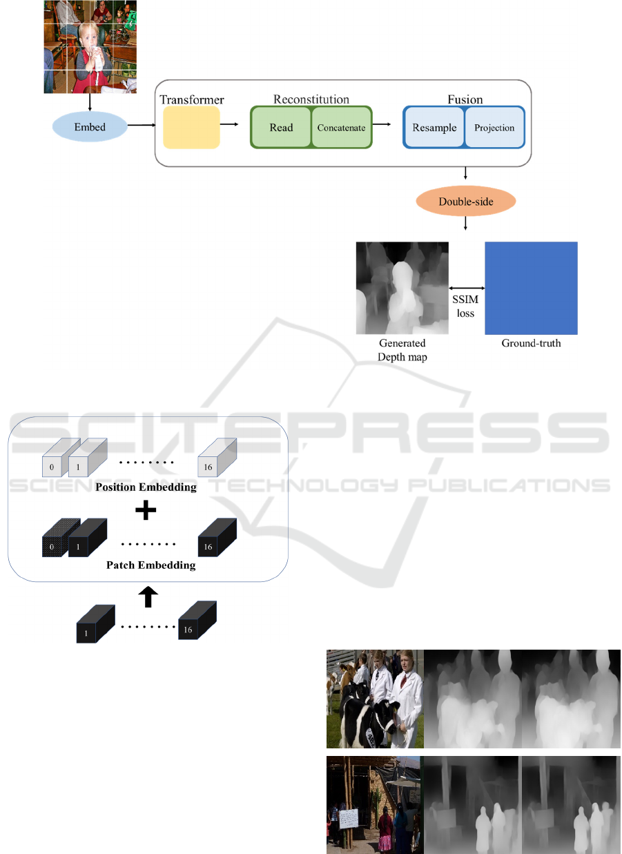
Figure 3: Proposed Method Overflow.

Figure 4: Transformer Position and Patch Embedding.

The Fusion module uses a repression similar to the

image of the Reconstitution block as an input as well

as the previous steps. It summarizes these two, applies

continuous convolution units, and then upsamples the

predicted repression. The presentation of the Fusion

module is used as an input to the Projection module.

The double-side consists of a small deconvolution

block with an upsampling module.

Finally, the loss value between the generated

depth map and the original Ground-truth is extracted

using SSIM. It is a function that evaluates quality in

three aspects: luminance, contrast, and structure. It

measure the similarity between the two images and

backpropagate through Impover to output a cleaner

and excellent Depth map.

5 EXPERIMENT AND

CONSIDERATIONS

The experimental result can be confirmed through

Figure 5. (a) is an input image, (b) is a Depth map

obtained using ViT, and (c) is an image outputting the

Depth map by applying the method proposed in this

study.

ISAIC 2022 - International Symposium on Automation, Information and Computing

154

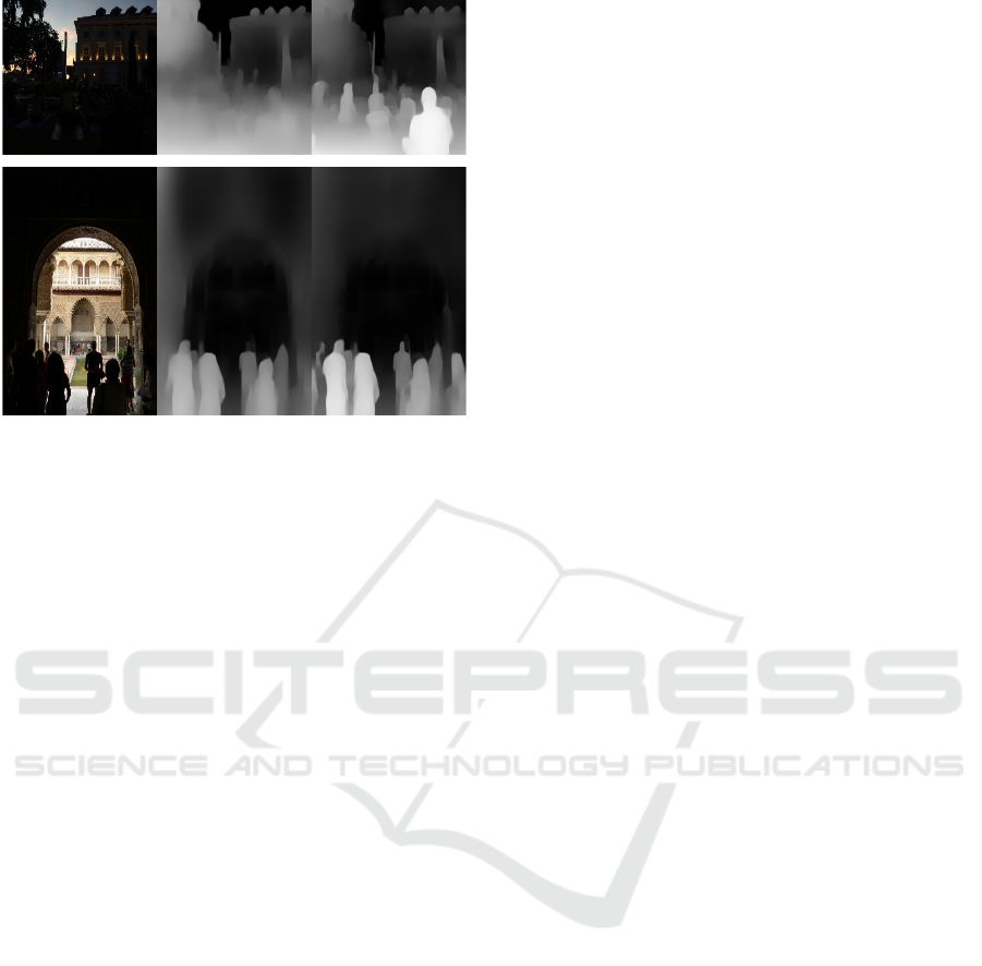
(a) (b) (c)

Figure 5: (a) input image (b) Depth map using ViT (c)

Depth map of the proposed method

In this paper, the 3D object in the image is

automatically focused using ViT and the Depth map

is output. It can be confirmed that the Depth map is

clean and accurate from the experimental result in

Figure 5. The automatically focused object in the

image is shown more intensely, and relative distance

from other nearby objects is accurately shown

through the proposed method. However, there is a

problem that the area is blurred and the overall image

quality is degraded since an area where two or more

objects overlap appears together without a boundary

between them.

REFERENCES

K. Alahari, G. Seguin, J. Sivic, and I. Laptev, “Pose

Estimation and Segmentation of People in 3D Movies,”

In Proc. IEEE International Conference on Computer

Vision, 2013.

Y.Lin, Z.Jun, and Y.Yingyun, “A Feature Extraction

Technique in Stereo Matching Network,” In Proc.

IEEE Electronic and Automation Control Conference,

2019.

Available: learnopencv.com/depth-estimationusing-stereo-

matching/

H. Baker and T. Binford, “Depth from Edge and Intensity

Based Stereo,” Proc. Int’l Joint Conf. Artificial

Intelligence, 1981.

A. W. Bergman, D. B. Lindell, and G. Wetzstein “Deep

Adaptive LiDAR: End-to-end Optimization of

Sampling and Depth Completion at Low Sampling

Rates,” IEEE Int. Conf. Comput. Photography,

pp. 1-11, 2020.

I. Alhashim and P. Wonka, “High Quality Monocular

Depth Estimation via Transfer Learning,” arXiv

preprint arXiv:1812.11941, 2018.

M.Y.Lee, C.H.Son, J.M.Kim, C.H.Lee, and Y.H.Ha,

“ Illumination-Level Adaptive Color Reproduction

Method with Lightness Adaptation and Flare

Compensation for Mobile Display,” Journal of

Imageing Science and Technology, Vol.51, No.1,

pp. 44-52, 2007.

G. Hongyun, T. Xin, S. Xiaoyong, and J.Jiaya, “Dynamic

Scene Deblurring with Parameter Selective Sharing

and Nested Skip Connections,” In IEEE, 2019.

P. Chae-rim, K. Jae-hoon, C. Seok-je, “Improving

Colorization Through Denoiser with MLP,” In

JAMET, pp. 1-7, 2022.

Alexey Dosovitskiy, Lucas Beyer and Alexander

Kolesnikov et al, “An Image is Worth 16x16 Words:

Transformers for Image Recognition at Scale,” ICLR

Published as a conference paper on Computer Vision

and Pattern Recognition, 2021.

Z. H Wang, AI. C Bovik, H. R. Sheikh, and E. P Simoncelli,

“Image Qulity Assessment: From Error Visibility to

Structural Similarity,” IEEE Transactions on Image

processing, pp. 600-612, 2004.

Depth Map Estimation of Focus Objects Using Vision Transformer

155