
Cooperative Trajectory Optimization for Long-Range Interception
with Terminal Handover Constraints
Zhengda Cui
1
, Mingying Wei
1,2
, Yunqian Li
1
and Pengfei Zhang
1
1
Beijing Institute of Electric System Engineering, Beijing 100854, China
2
Beijing Simulation Center, Beijing 100854, China
Keywords: Cooperative Handover Guidance, Long-range Interception, Cooperative Feasible Region, RBF Neural
Network.
Abstract: Motivated by the requirement of consistency engagement of long-range interceptors, a time cooperative
guidance method based on feasible region is proposed. First, the multi-missile cooperative trajectory planning
problem is established, considering the constraints in energy, heat protection and interception capacity. We
transform the problem into subproblems of determination of coordinated time and trajectory optimization
under time constraint. Based on the hp-adaptive pseudo-spectral method, the feasible region is analyzed and
solved under different initial conditions. The RBF neural network was used to realize the online negotiation
and prediction of cooperative cost. Numerical simulation shows the optimal cooperative trajectories can meet
the constraint on cooperative rendezvous.
1 INTRODUCTION
The conflict between air threat and interceptors is
becoming increasingly fierce in modern warfare, with
the range of precision-guided weapons getting farther
and farther. Interceptor missiles must also have the
ability to intervene quickly in remote areas and
accurately intercept various air targets (Wei, M, Cui,
Z, & Li, Y, 2020; Wang, F. B, & Dong, C. H, 2013;
Farooq, A, & Limebeer, D. J, 2002).
Unlike stationary or slow-moving targets, the
target set of long-range air-defense missiles also
includes high-mobility targets. Considering the long-
range and target maneuvers, the handover area
between midcourse and final interception is
inevitably expanded. In order to realize information
closure, it is used to add a trajectory planning phase
at the end of the midcourse phase, so that the positions
of multiple interceptors can meet the conditions of
cooperative detection field splicing, and improve the
capture probability of the seeker to the target.
The end stage of midcourse trajectory planning
problem for long-range air-defense missiles is often
described as a multi-constrained optimal control
problem under finite feasible regions (
GUO M,YANG
F,LIU K,XIA G,YANG J, 2022
); Because the
collaborative detection constraints are involved, it is
necessary to restrict the whole terminal state of the
interceptor, including position, velocity, velocity
angle and time. Meanwhile, the flight capability
boundary of each interceptor should be considered
comprehensively to find the cooperative trajectory
that meets the state and terminal constraints. With the
increase in the number of targets and interceptors,
finding such a trajectory under multiple constraints
via traditional method is time-consuming.
Considering the target movement, it is difficult to
meet the actual requirements of rapid response of
interceptors online.
There are nonlinear coupling among time,
speed, trajectory, constraint, and the horizontal and
longitudinal plane in the energy descent phase.
Nonlinear programming (NLP) tools can be used to
solve these problems (Lv, S, Cai, M, & Zhou, D,
2019). Besides, the numerical trajectory optimization
method can consider a variety of constraints and
directly use the dynamic model of interceptors, which
more truly reflects the mutual coupling between states
and the restraint relationship of air defense missiles
(Taub, I, & Shima, T, 2013).
In this paper, we study the coordination
rendezvous problem of long-range air-defense
missiles and trying to give a generalized structure to
realize the online negotiation and prediction of
cooperative cost. The key idea of this paper is to
divide the negotiation and optimization of the
trajectory into two subproblems: a) determination of
coordinated time and b) trajectory optimization under
Cui, Z., Wei, M., Li, Y. and Zhang, P.
Cooperative Trajectory Optimization for Long-range Interception with Terminal Handover Constraints.
DOI: 10.5220/0011917200003612
In Proceedings of the 3rd International Symposium on Automation, Information and Computing (ISAIC 2022) , pages 169-176
ISBN: 978-989-758-622-4; ISSN: 2975-9463
Copyright
c
2023 by SCITEPRESS – Science and Technology Publications, Lda. Under CC license (CC BY-NC-ND 4.0)
169

time constraint. And solve by nonlinear programming
tools. Based on the hp-adaptive pseudo-spectral
numerical optimization method, the properties of
feasible region are analyzed and fit the established
database with RBF neural network. Numerical
simulation shows the effeteness of the proposed
method.
2 PROBLEM STATEMENT
2.1 Dynamic Model
Assuming the vehicle is a point of mass, the kinetic
model of the
th
i
interceptor in the collaborative
mission is:
sin
cos
cos
cos cos
sin
cos sin
i
ii
i
i
ii
ii i
i
i
ii i
ii i i
ii i
iiii
D
Vg
m
Yg
mV V
Z
mV
xV
yV
zV
θ
θθ
ψ
θ
θ
ψ
θ
θ
ψ
=− −
=−
=−
=
=
=−
(0.1)
Where:
m ,
g
, V ,
x
, y , z are the mass, local
gravitational acceleration, velocity, position
components in the interceptor, respectively. The
local trajectory inclination angle
θ
is the angle
between the velocity vector and the local level, and
the heading angle
ψ
, that is, the angle between the
velocity vector and the local north direction.
Y ,
Z
,
D
are the lift, lateral force and resistance of the
interceptor; the control parameters
[
]
,
YZ
Uaa= is the
normal acceleration instruction in two directions, can
be expressed as follows:
Y
Y
a
m
=
,
Z
Z
a
m
= (0.2)
2.2 Boundary Conditions and
Constraints
Different from the re-entry trajectory planning
problem for hypersonic gliding vehicles, the main
feature of the long-range air-defense missile
collaborative trajectories planning problem lies in the
different constraints. Long-range air-defense missiles
use light body and axisymmetric layout, with lower
energy, smaller lift-drag ratio, thinner cylinder wall,
poorer heat resistance than the glide vehicle, and the
interception targets are high mobile aircraft targets.
Their unique constraints can be summarized as
follows:
I) Overload Constraints
Due to the axisymmetric layout of the air-defense
missiles, its high-altitude overload capability is very
limited, and the acceleration constraint of
aerodynamic steering missile can not be simply
considered as constant, but limited by the shell
structure and the aerodynamic capacity. The
maximum overload
maxT
n
for the shell structure can
be considered as the constant value, but the maximum
aerodynamic overload capacity is subject to
substantial aerodynamic pressure variation due to
altitude and speed change. So, it is coupled together
with speed, height and trajectory, it cannot be solved
analytically (Cho, S. B, & Choi, H. L, 2022). The
coupling relationship between overload constraints,
control history, and terminal constraints can be
expressed as the following formula:
[
]
1
,(,)
m
VfUt
ρ
= (0.3)
[
]
2lim
(, , ,)
f
Uf Ut= xx (0.4)
[
]
lim 3
(,)
m
UfV
ρ
= (0.5)
Where
x
refer to the state parameters,
lim
U
is
the time varying control limitation.
II) Detection Constraints
The multi-missile cooperative detection of long-
range air-defense missiles needs to create good
detection conditions for the seeker. It has strict
constraints on the position, difference in search time,
difference in speed, speed angle and lower bounds of
speed. They form the terminal constraints of long-
range air-defense missiles. In addition, the
interception object of air-defense missile interception
is the aircraft-class high dynamic maneuver target.
After the interceptor arrives in the handover area and
the seeker is started, the target may maneuver at any
time. The interceptor is required to have strong
maneuverability and the final speed as much as
possible, to reserve sufficient speed advantages and
overload capacity for the final guidance.
2.3 Optimization Problem
Transforming the problem of collaborative guidance
into optimal control is described as follows:
() ( )
min
()
Ut U
d
V
JU
∈Ω
=−
ISAIC 2022 - International Symposium on Automation, Information and Computing
170
min
lim
max
lim
max
12
s.t.
1, 2
ifi
ii
ii
ii
ii
ii
i
VV
UU
nn i N
UU
QQ
TT T
=
≥
≤
≤=
≤
≤
==…=
XX
(0.6)
()
T
,, ,,,
iiiiiii
XYZV
θψ
=X
Because of the nonlinearity aforementioned, the
optimization problem has no analytic solution. It can
only be solved via numerical methods.
3 FEASIBLE REGION FOR
COLLABORATIVE
DETECTION
As the number of interceptors in the bomb group
increases, the dimension explosion phenomenon will
appear, and it takes too long to solve the above
collaborative planning problem directly by numerical
methods. In order to give a general solution scheme
suitable for the arbitrary number of interceptors, this
paper divides the collaborative search problem into
two subproblems: solving the collaborative search
feasible region and constrained trajectory planning.
The difference between the collaborative search
feasible domain and the aircraft accessible
/recoverable region is that the former focuses on the
state-space boundary when the aircraft arrives at the
predicted handover point and focuses on its efficiency
on the subsequent mission; the latter focuses on the
space boundary of the aircraft, such as the hypersonic
aircraft foot print problem and the interceptor
interception area problem.
The Initial conditions are:
(0) 0X = ,
(0) 35 kmY =
,
(0) 0Z =
,
(0) 2000 /Vms=
,
(0) 0
θ
=°
,
(0) 0
ψ
=°
; The terminal conditions are:
() 200km
f
Xt = , ( ) 20km
f
Yt = , () 0
f
Zt = ,
() max
ff
Vt V= , () 0
f
t
θ
= , () 0
f
t
ψ
=°. For the
reason of retain the destruction ability to the target
after detection, the minimum value of the final speed
is limited as
( ) 1200 /
f
Vt m s≥ .
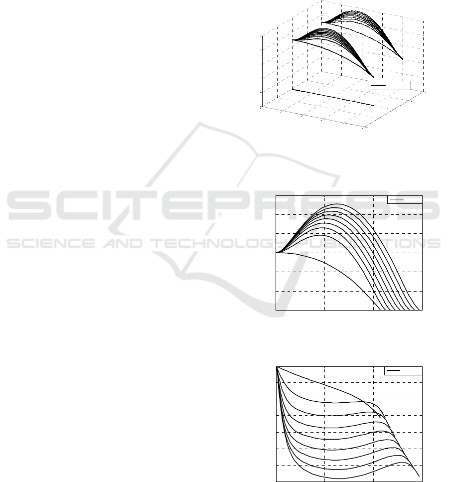
3.1 Unconstrained Feasible Region
The trajectory obtained without constraints is the
ideal scenario of the flight profile. Reflects the best
capability of the aerodynamic design of the aircraft.
In this paper, the maximum final speed trajectory and
the unconstrained feasible region are shown in Figure
1-4.
Figure 1: Unconstraint optimal trajectory for different
arrival time.
Figure 2: Height history.
Figure 3: Velocity history.
-20
-15
-10
-5
0
5
x 10
4
-1
-0.5
0
0.5
1
x 10
4
0
1
2
3
4
5
x 10
4
Z
X
Height
Traj ec tory
0 50 100 150
2
2.5
3
3.5
4
4.5
5
x 1 0
4
H / m
t / s
Height
0 50 100 150
1300
1400
1500
1600
1700
1800
1900
2000
V / (m/s)
t / s
Velocity
Cooperative Trajectory Optimization for Long-range Interception with Terminal Handover Constraints
171
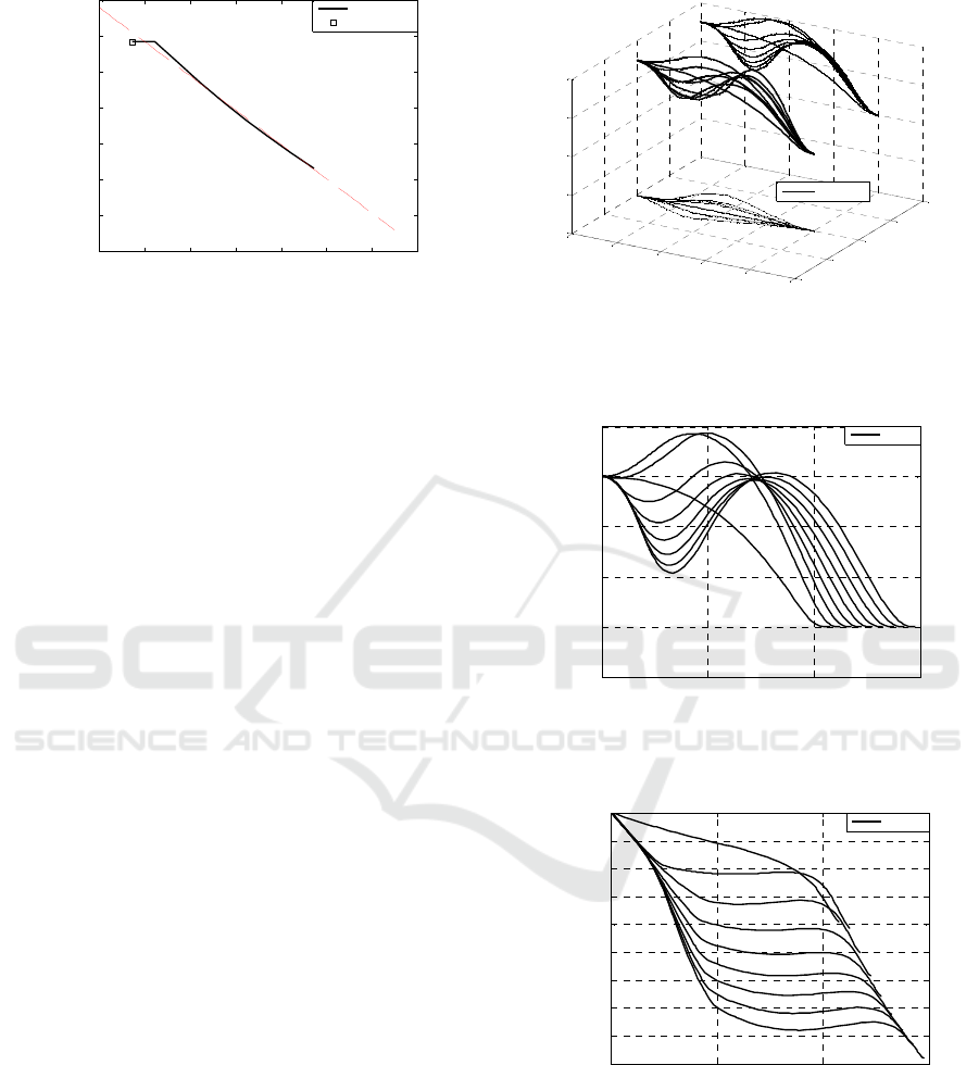
Figure 4: Maximum speed varies with time.
The simulation results show that after considering
the passive decay characteristics, the unconstrained
trajectory is only maneuver in the longitudinal plane.
The trajectories seem to be in the form of parabolic
trajectory. The former accomplishments related
mostly concentrate on the maximum terminal speed,
which is a critical factor for interception.
Nevertheless, this paper further points out through
simulation that the parabolic trajectory also can delay
the arrival time with minimum velocity cost. It has
certain reference significance for the subsequent
design of long-range air-defense missile coordinated
trajectories.
In addition, it can be seen that, after the maximum
speed can afford from parabolic trajectory, the speed
decreases while arrive time increases, and the linear
characteristics appear within a certain range. The
linear slope has obvious physical meaning: the
velocity cost of delay per second. This linear
correspondence will be further analyzed later.
3.2 Constrained the Feasible Region
After considering all the constraints of the long-range
air-defense missiles, the adjustable range of the shift
state is affected by the constraints, and it is reduced
accordingly. As shown in Figure 5~8:
Figure 5: Constrained optimal trajectory for different
arrival time.
Figure 6: Height history.
Figure 7: Velocity history.
100 110 120 130 140 150 160 170
1100
1200
1300
1400
1500
1600
1700
1800
t/s
V/ m/s
Upper bound
Minimum Time
-20
-15
-10
-5
0
5
x 10
4
-1
-0.5
0
0.5
1
x 10
4
0
1
2
3
4
x 10
4
Z
X
Height
Trajectory
0 50 100 150
1.5
2
2.5
3
3.5
4
x 10
4
H / m
t / s
Height
0 50 100 150
1100
1200
1300
1400
1500
1600
1700
1800
1900
2000
V / (m/s)
t / s
Velocity
ISAIC 2022 - International Symposium on Automation, Information and Computing
172
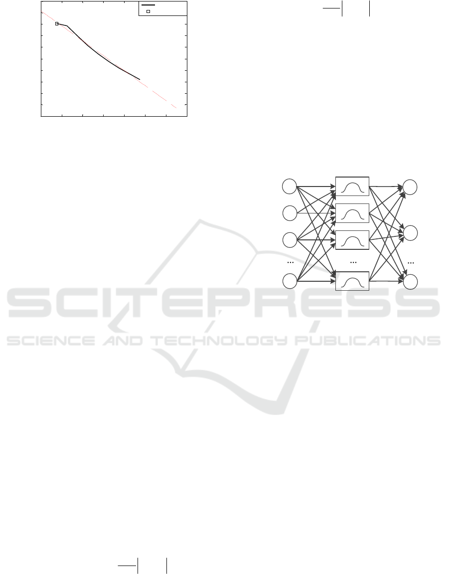
Figure 8: Maximum speed varies with time.
Compared with the unconstrained trajectory
above. It can be found that a) the trajectory changes
not only in the longitudinal plane, but also in the
horizontal plane. b) Because of the overload
limitation, the trajectory is in the form of double-
parabolic in the longitudinal plane, where only have
once in unconstrained scenario. c)
Maximum speed
varies with time still shows linear feature.
Furthermore, it is worth noticing that numerous
simulations show that it is unsensitive to the
disturbance on lift and drag coefficients, so it is
reasonable to fit the relationship linearly.
4 RBF NEURAL NETWORK
The Radical Basis Function (RBF) is one of the
multidimensional spatial interpolation techniques
proposed by Powell in 1985. In 1989, Jackson
demonstrated that RBF neural networks constructed
by RBF function as hidden layer neurons have the
ability to consistently approximate any nonlinear
continuous function. The RBF neural network has the
advantages of simple structure, explicit training
algorithm, and fast learning convergence. It is widely
used in the field of pattern recognition (Lampariello,
F, & Sciandrone, M, 2001) and nonlinear control
(Yang, H., & Liu, J, 2018)
.
The function commonly used in RBF neural
networks is Gaussian function, so the activation
function in a radial basis function neural network can
be expressed as:
()
2
2
1
exp
2
pi pi
i
Rx c x c
δ
−= − −
(4.1)
The neural network structured as Figure 9 can
get the output as:
2
2
1
1
exp
2
k
ii pi
i
i
yw xc
δ
=
=−−
12in=…,
(4.2)
Where,
()
12
,
p
pp
pn
x
xx x∈
is the p
th
input
sample,
i
c
is the node center of hidden layer,
ij
w
is the
connection weight between the hidden layer to the
output layer,
i
y
is the actual output of the i
th
node.
The solution of the feasible domain of the long-
range air-defense missile can be transformed into a
nonlinear function regression problem with six inputs
and three outputs. The input variables are: speed,
height, range, lateral deviation and two initial
deviation Angle, and the output variables are the
maximum speed, corresponding time and the slope K.
1
x
2
x
3
x
m
x
1
y
2
y
n
y
Input Layer Hidden Layer Output Layer
Figure 9: Schematic diagram of the RBF neural network.
The learning algorithm of the RBF neural
network needs to solve the problem having three
aspects, the center of the basis function, the variance,
and the weights between the hidden layer to the
output layer. using self-organized selection center
method as the training method for RBF neural
network. It can be divided into two stages, one is the
self-organized learning stage, this stage using K-
average clustering method determine the center
i
c
and variance
i
σ
, it is a nonlinear optimization
process; In second stage, in order to find the
appropriate weight for the output neurons, using
gradient descent method for training neurons in
output layer.
4.1 Training and Validation of RBF
Neural Network
Optimize 2700 sets of data points offline over the
possible range of initial conditions. The convergence
criteria of the loss function is set to be 4e-7, the
100 110 120 130 140 150 160 170
800
900
1000
1100
1200
1300
1400
1500
1600
1700
1800
t/s
V/ m/s
Upper bound
Minimum Time
Cooperative Trajectory Optimization for Long-range Interception with Terminal Handover Constraints
173
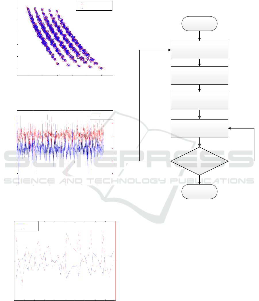
training and the testing result is shown in Figure
10~12:
Figure 10: RBF neural network fitting result.
Figure 11: Fitting error in RBF neural network.
Figure 12: Generalization capability of RBF neural
network.
4.2 Cooperative Guidance Strategy
Based on RBF Neural Network
The negotiation and optimization process of
consistency engagement as shown in Figure 13.
Trajectory tracking In cons ider
of modeling inaccuracies
Initial Conditons
Feasi ble region forecasting
based on RBF neural network
trajectory optimization under
time constraint
The tracking error is
within the allowable range
End
Y
N
Solve the cost of collaboration
and judg e whe ther it is
necessary to collaborate or not
Figure 13: Negotiation and optimization based on RBF
neural network.
5 SIMULATION RESULTS
The typical trajectory simulation of SM-6 missile is
given as an example, which satisfies all the
constraints and requirements on consistency
engagement. The initial parameters of the three
interceptors are shown in Table 1. And the forecast
results obtained through the neural network are
shown in Table 2. Because the time can only be
extended but not shorten, the coordination time is set
as (4.3), and the multiple interceptors plan their own
feasible trajectory. The planning results are shown in
Figure 14~16:
()
1
ma x , ,
f
ffi
ttt=…
(4.3)
0 0.2 0.4 0.6 0.8 1
0
0.2
0.4
0.6
0.8
1
Data Point
RBFNN Prediction
Training Value
0 500 1000 1500 2000 2500 3000
-3
-2
-1
0
1
2
3
Time fitting error
0 500 1000 1500 2000 2500 3000
-40
-30
-20
-10
0
10
20
Velocity fitting error
Time
Velocity
0 5 10 15 20 25 30 35 40 45 50
-0.5
0
0.5
Precision of time prediction
0 5 10 15 20 25 30 35 40 45 50
-5
0
5
Precision of velocity prediction
Time
Velocity
ISAIC 2022 - International Symposium on Automation, Information and Computing
174
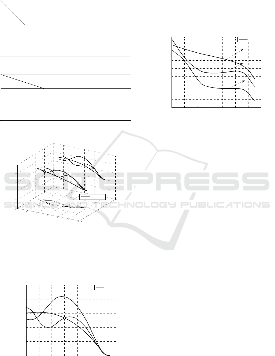
Table 1: Initial conditions of the interceptors.
Trajectory
Parameter
Missile
Number
0
L
R
0
θ
0
h
0
V
0
Z
0
ψ
1
M
240km
1°
35km 2000m/s 300m
2°
2
M
200km
1−°
37km 1930m/s 500m
2−°
3
M
220km
2−°
33km 2070m/s 0m
0°
Table 2: Forecast results of the RBF neural network
Trajectory Parameter
Missile Number
f
t
f
V
K
1
M
131.1 s 1558.9 m/s -9.25
2
M
111.2 s 1541.2 m/s -12.6
3
M
117.1 s 1586.9 m/s -10.4
According to the formula (4.3), we can get
131.1
f
ts=
Figure 14: Cooperative trajectory for different interceptors.
Judging by the trajectory, all the interceptors
can reach the target with terminal constraints. And
they maneuver in both the horizontal and
longitudinal planes.
Figure 15: Height varies with time.
In longitudinal planes,
3
M
’s trajectory is in
the form of single high-parabolic ballistics, and
2
M
’s is in the form of double-parabolic. They both
extend the encounter time while reducing terminal
speed losses.
Figure 16: Velocity varies with time.
The optimal cooperative trajectories and can
satisfied the constraints and can adjust the terminal
time to realize the collaborative rendezvous of all
interceptors.
6 CONCLUSIONS
This paper proposes a method of time cooperative
guidance method based on feasible region to meet the
collaborative rendezvous problem for long-range air-
defense missile. First, the trajectory optimization
problem is decomposed into two subproblems of
determination of the coordinated time and trajectory
optimization under time constraint. Based on hp-
adaptive pseudo-spectral based solution, RBF neural
networks were trained to realize the online
negotiation and prediction. Trajectory simulation
shows that the proposed method can quickly negotiate
the terminal conditions and realize the multi-missile
cooperative planning for long-range air-defense
missiles.
REFERENCES
Wei, M., Cui, Z., & Li, Y. (2020). Review and future
development of multi-missile coordinated interception.
Acta Aeronautica et Astronautica Sinica, 41(suppl 1)),
29-36.
-2.5
-2
-1.5
-1
-0.5
0
0.5
x 10
5
-1
-0.5
0
0.5
1
x 10
4
0
1
2
3
4
5
x 10
4
Z
X
Height
Trajectory
0 20 40 60 80 100 120 140
2
2.5
3
3.5
4
4.5
x 10
4
H / m
t / s
Height
0 20 40 60 80 100 120 140
1200
1300
1400
1500
1600
1700
1800
1900
2000
2100
V / (m/s)
t / s
Velocity
tf=131.1 s
Vf=1464 m/s
tf=131.1 s
Vf=1557 m/s
tf=131.1 s
Vf=1286 m/s
Cooperative Trajectory Optimization for Long-range Interception with Terminal Handover Constraints
175

Wang, F. B., & Dong, C. H. (2013). Fast intercept trajectory
optimization for multi-stage air defense missile using
hybrid algorithm. Procedia Engineering, 67, 447-456.
Farooq, A., & Limebeer, D. J. (2002). Trajectory
optimization for air-to-surface missiles with imaging
radars. Journal of guidance, control, and dynamics,
25(5), 876-887.
GUO Mingkun,YANG Feng,LIU Kai,XIA
Guangqing,YANG Jingnan. (2022). Research progress
of collaborative guidance technology of hypersonic
aircraft[J].Aerospace Technology, (02):75-84.
Shoukun, L. V., Mingchun, C. A. I., Di ZHOU, Z. H. O. U.,
& Zicai, W. A. N. G. (2019, July). Trajectory
optimization for Long-Range Air-Defense Missile with
a Constraint on Capability of Error Correction. In 2019
Chinese Control Conference (CCC) (pp. 3804-3808).
IEEE.
Taub, I., & Shima, T. (2013). Intercept angle missile
guidance under time varying acceleration bounds.
Journal of Guidance, Control, and Dynamics, 36(3),
686-699.
Cho, S. B., & Choi, H. L. (2022). A Convex Programming-
Based Approach to Trajectory Optimization for
Survivability Enhancement of Homing Missiles.
International Journal of Aeronautical and Space
Sciences, 1-17.
Wang, X., Zhang, Y., Liu, D., & He, M. (2018). Three-
dimensional cooperative guidance and control law for
multiple reentry missiles with time-varying velocities.
Aerospace Science and Technology, 80, 127-143.
Wen, L. I., Teng, S. H. A. N. G., Yinwei, Y. A. O., & Qilun,
Z. H. A. O. (2020). Research on time-cooperative
guidance of multiple flight vehicles with time-varying
velocity. Acta armamentarii, 41(6), 1096.
Liu, Z., Zheng, W., Wang, Y., Wen, G., Zhou, X., & Li, Z.
(2020, November). A cooperative guidance method for
multi-hypersonic vehicles based on convex
optimization. In 2020 Chinese Automation Congress
(CAC) (pp. 2251-2256). IEEE.
Zhou, H., Wang, X., & Cui, N. (2020). Glide guidance for
reusable launch vehicles using analytical dynamics.
Aerospace Science and Technology, 98, 105678.
Huang, G. B., Saratchandran, P., & Sundararajan, N.
(2005). A generalized growing and pruning RBF
(GGAP-RBF) neural network for function
approximation. IEEE transactions on neural networks,
16(1), 57-67.
Yingwei, L., Sundararajan, N., & Saratchandran, P. (1998).
Performance evaluation of a sequential minimal radial
basis function (RBF) neural network learning
algorithm. IEEE Transactions on neural networks, 9(2),
308-318.
Lampariello, F., & Sciandrone, M. (2001). Efficient
training of RBF neural networks for pattern
recognition. IEEE transactions on neural networks,
12(5), 1235-1242.
Yang, H., & Liu, J. (2018). An adaptive RBF neural
network control method for a class of nonlinear
systems. IEEE/CAA Journal of Automatica Sinica,
5(2), 457-462.
ISAIC 2022 - International Symposium on Automation, Information and Computing
176
