
Multivariate Analysis for Main Quality
Variable Control in Industry 4.0
Jorge M. de Souza
a
, Fabrício Cristófani
b
and Giovanni M. de Holanda
c
FITec - Technological Innovations, Aguaçu street, Campinas, Brazil
Keywords: Multivariate Analysis, Quality Control, Industry 4.0, out-of-Control, Out-of-Quality.
Abstract: The T
2
Hotelling one-dimensional control chart representation points out the out-of-control samples but does
not display how the secondary variables affects the primary ones considered the main quality variable. From
the same depart, the CHI squared distribution, a 2nd degree equation is derived highlighting the main quality
variable and its dependence on the secondary ones. This approach allows the identification of out-of-control
points that affects quality and require some adjustment of the secondary variables and the out-of-quality points,
which need an investigation of the root causes that lead to this undesirable output.
1 INTRODUCTION
With the technological innovations made possible by
the resources of Industry 4.0, quality control
techniques for production processes can and should
be refined to keep pace with these changes. Engineers
and manufacturing process supervisors can benefit,
for example, from clearer and more interactive
assessments of sample data generated in
manufacturing production (Godina and Matias,
2019). These issues have been presented either as a
requirement for the sustainable performance of the
industry (Foidl and Felderer, 2016) and to leverage
predictive actions resulting from a more
instrumentalized quality control–see, for example,
(Lee et al., 2019).
Indeed, in several industries, semiconductor,
metallurgy, cosmetics etc. there are one or more main
quality variables that quantify the product quality
(piston ring diameter, solution purity etc.) that are
affected by secondary ones that should be
investigated when the quality goal is not reached
(Palací-Lopez et al., 2020). These goals can be
achieved with stable and well-controlled processes. In
this sense, increased quality is defined as a reduction
in the variability of processes and products, which can
a
https://orcid.org/0000-0002-9902-6547
b
https://orcid.org/0000-0003-0142-2179
b
https://orcid.org/0000-0001-5603-2675
make of statistical methods essential in efforts to
improve processes (May and Spanos, 2006).
As each stage of the manufacturing process has a
set of variables whose measurements and control
involve a defined number of observations, statistical
models are used to monitor deviations of these
parameters and thus exercise forms of control to
detect process variability and its impact on the
product quality. In practice, many factors can
influence such a variability as improperly adjusted or
controlled machines, operator errors, different
operators crew, defective raw material, temperature
variation etc. that contribute to increase this
variability and increase the production of non-
conforming items.
The way these variables are measured is shifting
with the Industry 4.0 with the possibility to record
100% of measured data by means of IoT sensors and
wireless network (Godina and Matias, 2019). This
huge amount of data must be classified to consider the
many factors that can influence the variability as
pointed previously.
Therefore, in the context of Industry 4.0 it is
necessary the simultaneous statistical control of two
or more quality characteristics making possible to
266
M. de Souza, J., Cristøsfani, F. and M. de Holanda, G.
Multivariate Analysis for Main Quality Variable Control in Industry 4.0.
DOI: 10.5220/0011921600003612
In Proceedings of the 3rd International Symposium on Automation, Information and Computing (ISAIC 2022), pages 266-272
ISBN: 978-989-758-622-4; ISSN: 2975-9463
Copyright
c
2023 by SCITEPRESS – Science and Technology Publications, Lda. Under CC license (CC BY-NC-ND 4.0)
control the impact of variability. In this context,
multivariate control charts (MCC) are used in the
aggregated monitoring of two or more process or
product variables. The p-dimensional points (that is,
the values of p random variables or statistics of
interest derived from them) are represented one-
dimensionally and presented in graphs similar to
Shewhart charts, simplifying the task of simultaneous
control of variables.
The paper is structured as follows: In Section 2,
the motivation for this approach is presented,
highlighting how multivariate analysis can bring new
information for process monitoring and control, and
how to specify control limits based on capability
index. Section 3 presents the ellipse control
expressions for multivariate analysis. Section 4 is
dedicated to the T
2
Hotelling approach. Finally, in the
Section 5, the method proposed is applied to three
variables highlighting the concept of out-of-control
and out-of-quality points.
2 WHY MULTIVARIATE
ANALYSIS? THE MOTIVATION
Industry 4.0 will allow at low cost a significant spread
of sensor technology on shop floors gathering a huge
volume of data. New levels of quality control have
been demanded to match the current abundance of
data and the facilities made possible by new
automation and data intelligence technologies, in a
way to extract more effective value from this new
production management potential–see, for example,
(Moyne and Iskandar, 2017), (Lee et al., 2019).
The resources of statistical process control, which
have been applied for a long time in the productive
environment, are also gaining state-of-the-art studies
and becoming more specialized to further contribute
to the quality management (Zhong et al., 2017), (Tu
et al., 2009), (Sindhumol et al., 2018). Some
approaches include cutting-edge technological
solutions, for example neural network in a system to
detect and classify fabric defects (Mahmud et al.,
2021), which even though not within the scope of
statistical control, illustrates the efforts applied to
improve quality control practices in view of the news
demands of the Industry 4.0.
When it comes to the production of
semiconductors–such as solid-state drive (SSD) and
multi-chip packages, to name a few types–, which can
involve multistage and multistep processes, many
factors can influence the quality of the production
process in an aggregated and interdependent way.
Several techniques have been used to analyze the
multiple variables acting in this process, with
approaches that try to capture the process
particularities, monitor the control limits established
for production and deepen the analyses to increase the
interpretability of the collected data.
By focusing on a timeline of the technical
literature of this century, one can observe that two
decades ago, (Skinner et al.,2002) already compared
multivariate statistical methods to analyze wafer data.
A few years later, based on multivariate analysis, (Ma
et al., 2010) extracted key variables from a broad set
of variables measured with small number of runs.
Currently, amidst the challenges of big data in
semiconductor production, (Saib et al., 2021) presents
a multivariate analysis method for large amounts of
multidimensional data. Already (Chien and Chen,
2021) developed a collinear multivariate model-
based approach to extend managerial capabilities in
intelligent semiconductor manufacturing.
In this context, there is an issue that quality
management may have multivariate quality control
tools to detect the variations among data that are not
independent. In other words, data should be jointly
considered, otherwise the quality management
analysis can lead to erroneous conclusions. Another
issue is how to show the way secondary variables
affects primary ones.
This second point is the motivation of this paper.
We propose to consider a practical example to
highlight the proposition.
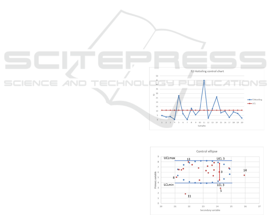
Figure 1: T2 Hotelling control chart.
Figure 2: X-Y Control ellipse. Sample 3 control limits.
Figure 1 shows the T
2
Hotelling control chart
analyzing two variables. Figure 2 displays the X-Y
Multivariate Analysis for Main Quality Variable Control in Industry 4.0
267
dispersion of the variables and the ellipse multivariate
control chart.
The samples 5, 11 and 14 are out-of-control points
but a difference can be pointed. The value of the
secondary variable of sample 14 is within the
maximum control limits of the primary variable and
can be adjusted to be inside the ellipse to ensure
primary variable control. Differently, the same does
not happen with the value of the secondary variable
of samples 5 and 11 that are out of the maximum
control limits of the primary variable directly
affecting the quality.
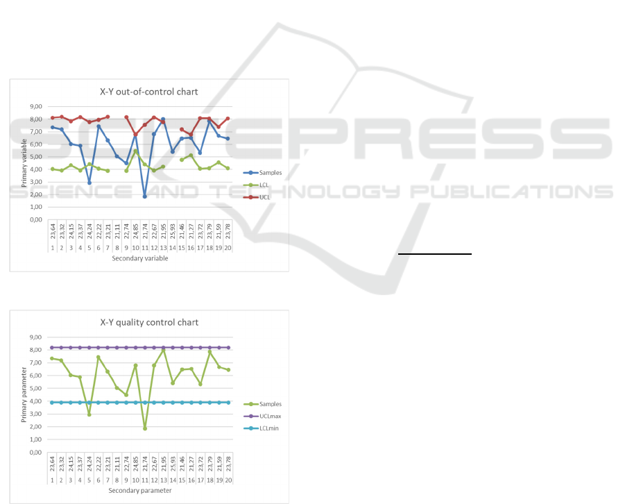
The ellipse control chart is not easily visualized
when several secondary variables are considered,
since is difficult to construct the ellipse for more than
two quality variables. It is proposed a X-Y control
chart, as illustrated in Figures 3 (a) and (b) for two
variables. The UCL, Upper Control Limit and LCL,
Lower Control Limit are the intersection of the
vertical straight-line of each sample with the ellipse
curve, changing with the time sequence of the
samples. The break of the UCL and LCL limits at
samples 8 and 14 is explained by the lack of solution
because they not vertically intersect the ellipse.
Figure 3(a): X-Y Out-of-control chart.
Figure 3(b): X-Y quality control chart.
The X-Y quality control chart points out the
samples that are not inside the quality range
delimitated by UCLmax and LCLmin, which
respectively represent the maximum of the UCL
values and the minimum of the LCL values shown in
figure 3(a)
For more than two secondary variables, the set
will be displayed by a table.
In the following sections the ideas herein
presented are developed.
3 ELLIPSE CONTROL CHART
Equation (1) is the matrix exponent of the
multivariate normal density function.
𝑋
−𝑋
𝑆
𝑋
−𝑋
(1
)
where:
𝑋
= 𝑋
,𝑋
,
...𝑋
is the mean vector of the p
variables,
𝑋
= the mean vector of means
and S the matrix of covariances.
Suppose that p quality variables are jointly
distributed according to the bivariate normal
distribution with sample averages of the quality
variables computed from a sample of size n, then the
statistics
𝜒
,
=𝑛𝑋
−𝑋
𝑆
𝑋
−𝑋
(2)
will have a chi-square distribution with p degrees of
freedom.
Let 𝜒
,
be the upper
α
percentage point of the
chi-square distribution with p degrees of freedom
For p=2 the following equations holds:
𝜒
,
=𝑛
1
𝜎
𝜎
−𝜎
𝜎
𝑣
+ 𝜎
𝑣
−2𝑣
𝑣
𝜎
(3)
𝑣
= 𝑋
−𝑋
𝜎
𝑣𝑎𝑟𝑖𝑎𝑛𝑐𝑒 𝑜𝑓 𝑖,𝜎
𝑐𝑜𝑣𝑎𝑟𝑖𝑎𝑛𝑐𝑒 𝑏𝑒𝑡𝑤𝑒𝑒𝑛 𝑖,𝑗
Equation (3) is the base of the ellipse control
example of Figure 2 taking variable 1 as primary and
2 as secondary for a given n and α.
For p variables, taking p = 1 as the primary one,
the equation (2) can be expressed as:
𝜒
,
=𝑛
𝑣
𝑉
,
𝜎
𝑆
,
𝑆
,
𝑆
,
𝑣
𝑉
,
(4)
𝑉
,
,𝑆
,
𝑠𝑢𝑏𝑎𝑟𝑟𝑎𝑦 𝑜𝑓 𝑖 𝑙𝑖𝑛𝑒𝑠 𝑎𝑛𝑑 𝑗 𝑐𝑜𝑙𝑢𝑚𝑛𝑠
Expression (4) is a 2
nd
degree equation for
variable 1.
ISAIC 2022 - International Symposium on Automation, Information and Computing
268

4 THE MULTIVARIATE
APPROACH
Generally, MCC (Multivariate Chart Control) are
used in situations where there is a significant
correlation between the variables to be monitored,
since in most of the multivariate processes the
variables interfere and suffer interference with each
other, thus having a strong correlation. In addition,
these charts are useful in cases where the variables are
not correlated, as they are capable of monitoring
processes in which there is a possibility of false
alarms when the operator finds problems in a certain
variable that is not necessarily interfering with the
process. According to (Montgomery, 2013), the
difference between univariate and multivariate
control is the increase in the complexity and levels of
automation of production processes, together with the
collaboration of growing computational support.
For (Mason and Young, 2001), a control
procedure based on Hotelling's T
2
statistics observes
the fact that a change in a variable can cause a ripple
effect throughout a system. By considering the
interrelationships between variables, the T
2
statistics
produces a powerful tool that is useful in detecting
subtle changes in the system. This fact explains the
expansion of multivariate control within industries,
simultaneously monitoring the various quality
characteristics (process variables)–see, for example,
the application of (Tavares and Ramos, 2006) in the
Brazilian aluminum industry, and (Nunes et al.,2018)
discuss the use of this and other multivariate control
charts in industrial processes with automatization and
large data volumes.
The most popular multivariate control charts are
the Chi-squared and Hotelling’s T
2
charts. They
follow the same line of the univariate Shewhart chart
and can detect large variations in the process along
with its behavior related to its mean. The Chi-squared
control chart considers that the vector of the mean of
the characteristics and the covariance matrix of the
variables involved are known. We know that in
practice this almost does not happen. Thus, in our
approach, we considered the Hotelling’s T
2
chart,
since it uses assumptions that are estimated by means
of preliminary samples collected from the process,
when it is under statistical control.
Now, we present a summary of the ideas about
Hotelling’s T
2
charts contained in (Montgomery,
2013), in order to formalize it. The T
2
chart was
developed by Hotelling in 1947, which was a pioneer
researcher on multivariate control charts. In formal
terms, to build the chart, the quadratic form expressed
in equation (5) is considered:
𝑇
=𝑛𝑋
−𝑋
𝑆
𝑋
−𝑋
(5)
Being more specific, for each line k of the sample
and each characteristic j, it is considered that
𝑋
=
1
𝑛
𝑋
(6)
𝑠
=
1
𝑛−1
𝑋
−𝑋
(7)
In both equations, (6) and (7), 𝑗=1,2,...,𝑝 and
𝑘=1,2,...,𝑚. While the covariance between
features j and h at the k-th coordinate is given by
equation (8)
𝑠
=
1
𝑛−1
𝑋
−𝑋
𝑋
−𝑋
(8)
with 𝑘 =1,2,...,𝑚 and 𝑗≠ℎ. Consequently,
𝑋
and S are obtained considering the averages
𝑋
=
1
𝑚
𝑋
,𝑗=1,2,…,𝑝
𝑠̅
=
1
𝑚
𝑠
,
𝑗=1,2,…,𝑝
𝑠
̅
=
1
𝑚
𝑠
,𝑗≠ℎ
(9)
and the matrix.
𝑆=
𝑠
̅
⋯𝑠
̅
⋮⋱⋮
𝑠
̅
⋯𝑠
̅
(10)
It is important to note that, in this case, 𝑋
represents the elements of vector 𝑋
𝑒 𝑆 represents the
covariance matrix considering the mean of the
covariance of each line of the sample.
The construction of Hotelling’s T
2
chart has two
distinct phases. Phase I consists of using the graph to
test whether the process was under control when the
first observations were extracted. In this case, the
objective is to obtain a set of data under control for
establishing the control limits. Phase II, in turn, uses
these limits to test whether the process remains under
control, when future observations are extracted.
Upon completion of the Phase I, the limits are
defined as expressed in equations (11) and (12)
𝑈𝐶𝐿 𝐼 =
𝑝
𝑚−1
𝑛−1
𝑚𝑛−𝑚−𝑝+1
𝐹
,,
(11)
𝐿𝐶𝐿 𝐼= 0
(12)
where p is the number of characteristics being
considered simultaneously, n is the size of the
subgroup, m is the total of samples and
Multivariate Analysis for Main Quality Variable Control in Industry 4.0
269

𝐹
,,
is a point of a portion of the upper
percentage of the F distribution with p and 𝑚𝑛−
𝑚−𝑝+1 degrees of freedom. For the case in which
future observations are extracted from the process, in
Phase II, the control limits are calculated via
equations (13) and (14)
𝑈𝐶𝐿 𝐼𝐼=
𝑝
𝑚+1
𝑛−1
𝑚𝑛−𝑚−𝑝+1
𝐹
,,
(13)
𝐿𝐶𝐿 𝐼𝐼= 0
(14)
where p, m and n represent the same parameters
defined previously. When a large number of samples
is considered, it is customary to use 𝑈𝐶𝐿=𝜒
,
as
the upper control limit in both phases I and II. In this
case, 𝜒
,
represents the upper percentage point of
the Chi-squared distribution with 𝑝 degrees of
freedom–see (Montgomery, 2013) for more details.
5 APPLICATIONS
A hypothetical example is considered to exemplify
the proposed multivariate analysis.
Table 1: Samples.
Sample
𝑋
𝑋
𝑋
1 23.64 7.34 5.18
2 23.32 7.18 3.78
3 24.15 6.04 5.32
4 23.37 5.88 4.72
5 24.24 2.94 4.50
6 22.22 7.44 4.24
7 23.21 6.30 6.44
8 21.11 5.04 5.22
9 22.74 4.50 4.66
10 24.85 6.80 6.04
11 21.74 1.85 5.36
12 22.67 6.81 5.06
13 21.95 8.00 3.32
14 25.93 5.42 3.78
15 21.46 6.46 3.40
16 21.27 6.51 5.20
17 23.72 5.33 5.38
18 23.79 7.85 7.46
19 21.59 6.66 5.32
20 23.78 6.44 4.46
𝑋
23.03 6.04 4.94
Table 1 shows the mean of the variables
considering n = 5, m = 20 and p = 3. Primary variable
1 is dependent of the other two secondary variables.
The T
2
Hotelling chart points out eight out-of-
control points as shown in figure 3.
Figure 4: T
2
Hotelling chart.
The X-Y chart based on equation (4) highlights
the out-of-controls points but also those that directly
affects the primary variable which measure the output
quality. The control limits UCL and LCL shown in
Figure 5 are time-varying with the sample sequence,
since they represent the intersection of the vertical
straight-line of each sample with the ellipse curve, as
explained in Section 2. In Figure 6, the X-Y quality
control chart points out the samples that are not inside
the quality range delimitated by UCLmax and
LCLmin, which respectively represent the maximum
of the UCL values and the minimum of the LCL
values shown in figure 5
Figure 5: Out-of-control chart.
Figure 6: Quality control chart.
ISAIC 2022 - International Symposium on Automation, Information and Computing
270

The control limits UCL/LCL enclose the out-of-
control points and UCLmax/LCLmin delimit the
quality control area, concerning the primary variables
whose limits are determined by the secondary ones.
Sample 14 can be considered an out-of-quality point
and Table 1 displays the values of the secondary
variables which lead to this nonconformity. In other
words, the out-of-control points need a correct setting
of the secondary variables, but the out-of-quality
points need an investigation of the root causes that
lead to this output.
6 CONCLUSIONS
In many applications concerning quality control in
Industry 4.0 there are sensors that measure the output
quality variables and those that measure the
secondary variables affecting the output quality. A
quality control analysis should take this particularity
into account.
Due to correlation between measured variables in
the industrial process Multivariate analysis is of
paramount importance because individual variable
control can lead to erroneous conclusions.
Multivariate analysis based on the T
2
Hotelling is
a one-dimensional control chart representation
pointing out the out-of-control samples but does not
display how the secondary variables affects the
primary ones, considered the main quality variables.
Based on the Chi-squared distribution, a 2
nd
degree equation is derived highlighting the main
quality variable and its dependence on the secondary
ones. This approach allows the identification of out-
of-control points that affects quality and require some
adjustment of the secondary variables and the out-of-
quality points, which need an investigation of the root
causes that lead to this undesirable output.
For further work, we planned to include data
assimilation into the statistical modelling and
consider predictive uncertainty quantification in this
approach, with the purpose of evaluating to what
extension this analytical detailing will contribute to
support more assertive decisions. Such an evaluation
might be feasible, as long as we have a significant
increase in the amount of monitored data.
ACKNOWLEDGEMENTS
The authors would like to thank the Brazilian
Ministry of Science, Technology and Innovations for
the financial support part of this project through the
PADIS (Program of Support for the Technological
Development of the Semiconductor and Displays
Industry).
REFERENCES
Chien, C.-F., Chen, C.-C. (2021) Adaptative parametric
yield enhancement via collinear multivariate analytics
for semiconductor intelligent manufacturing. Applied
Soft Computing, 108.
https://doi.org/10.1016/j.asoc.2021.107385
Foild, H., and Felderer, M. (2016) Research Challenges of
Industry 4.0 for Quality Management. International
Conference on Enterprise Resource Planning Systems,
In: Felderer M., Piazolo F., Ortner W., Brehm L., Hof
HJ. (eds) Innovations in Enterprise Information
Systems Management and Engineering. ERP Future
2015. Lecture Notes in Business Information
Processing, vol 245. Springer, Cham.
https://doi.org/10.1007/978-3-319-32799-0_10
Godina R., Matias J.C.O. (2019) Quality Control in the
Context of Industry 4.0. In: Reis J., Pinelas S., Melão
N. (eds) Industrial Engineering and Operations
Management II. IJCIEOM 2018. Springer Proceedings
in Mathematics & Statistics, vol 281. Springer, Cham.
https://doi.org/10.1007/978-3-030-14973-4_17
Lee, S.M., Lee, D. & Kim, Y.S. (2019) The quality
management ecosystem for predictive maintenance in
the Industry 4.0 era. Int J Qual Innov 5, 4.
https://doi.org/10.1186/s40887-019-0029-5
Ma, M.-D, Wong, D.S.-H., Jang, S.-S., Tseng, S.-T. (2010)
Fault detection based on statistical multivariate analysis
and microarray visualization. IEEE Transactions on
Industrial Informatics, 6 (1), 18-24. Doi:
10.1109/TII.2009.2030793
Mahmud T., Sikder J., Chakma R.J., Fardoush J. (2021)
Fabric Defect Detection System. In: Vasant P., Zelinka
I., Weber GW. (eds) Intelligent Computing and
Optimization. ICO 2020. Advances in Intelligent
Systems and Computing, 1324. Springer, Cham.
https://doi.org/10.1007/978-3-030-68154-8_68
Mason, R. L.; Young, J. C. (2001) Multivariate Statistical
Process Control with Industrial Application.
Philadelphia: Society for Industrial and Applied
Mathematics.
May, G. S.; Spanos, C. J. (2006). Fundamentals of
semiconductor manufacturing and process control.
New Jersey: Wiley-Interscience.
Montgomery, D. (2013) Introduction to statistical quality
control. New York: John Wiley & Sons.
Mottonen, M., Belt, P., Harkonen, J., Haapasalo, H., Kess,
P. (2008) Manufacturing Process Capa-bility and
Specification Limit. The Open Industrial and
Manufacturing Engineering Journal, 1, 29-36.
Moyne, J., Iskandar, J. (2017) Big data analytics for smart
manufacturing: Case studies in semicon-ductor
manufacturing. Processes 2017, 5 (39).
Doi:10.3390/pr5030039
Multivariate Analysis for Main Quality Variable Control in Industry 4.0
271

Nunes, T.F.B., Carrir, R.C., Rosa, A.F.P., Royer, R. (2018)
Parametric multivariate control charts: a review.
RAUnP, 10 (3).
https://doi.org/10.21714/raunp.v10i3.1836
Palací-Lopez, D., Borràs-Ferrís, J., Oliveria, L.T.S., Ferrer,
A. (2020) Multivariate Six Sigma: A Case Study in
Industry 4.0. Processes 2020, 8, 1119;
Doi:10.3390/pr8091119
Saib, M., Lorusso, G. F, Charley, A.-L., Leray, P., Kondo,
T., Kawamoto, Y., Ebizuka,Y., and Ban, N. (2021)
Multivariate analysis methodology for the study of
massive multidimensional SEM data. Proc. SPIE
11611, Metrology, Inspection, and Process Control for
Semiconductor Manufacturing XXXV, 116112C.
https://doi.org/10.1117/12.2583696
Sindhumol, M.R., Gallo, M., Srinivasan, M.R. (2018)
Monitoring Industrial Process using a Ro-bust
Modified Mean Chart”, Austrian Journal of Statistics,
48 (1), pp. 1-13. Doi:10.17713/ajs.v48i1-1.765
Skinner, K.R., Montgomery, D.C., Runger,G.C., Fowler,
J.W., McCarville, D.R., Rhoads, T.R., and Stanley, J.D.
(2002) Multivariate statistical methods for modeling
and analysis of wafer probe test data. IEEE
Transactions on Semiconductor Manufacturing, 15 (4),
523-530. Doi: 10.1109/TSM.2002.804901
Souza J.M., Holanda G.M., Henriques, H.A., Furukawa
R.H. (2021) Modified Control Charts Monitoring
Long-Term Semiconductor Manufacturing Processes.
In: Iano Y., Saotome O., Kemper G., Mendes de Seixas
A.C., Gomes de Oliveira G. (eds) Proceedings of the
6th Brazilian Technology Symposium (BTSym’20).
BTSym 2020. Smart Innovation, Systems and
Technologies, vol 233. Springer, Cham.
https://doi.org/10.1007/978-3-030-75680-2_11
Tavares, P.S., Ramos, E.M.L.S. (2006) Gráfico de controle
multivariado T2 de Hotelling - instrumento de análise
da qualidade numa indústria de alumínio. SPOLM
2006, 539-550.
Tu, K.K.-W, Lee, J.C.-S., and Lu, H.H.-S. (2009) A Novel
statistical method for automatically partitioning tools
according to engineers’ tolerance control in process
improvement. IEEE Transactions on Semiconductor
Manufacturing, 22 (3), 373-380. Doi:
10.1109/TSM.2009.2025812
Yang, C., Chang, C.-J., Niu H.-J.& Wu, H.-C. (2008)
Increasing detectability in semiconductor foundry by
multivariate statistical process control. Total Quality
Management & Business Excellence, 19 (5), 429-440.
Doi: 10.1080/14783360802018079
Zhong, R. Y., Xu, X., Klotz, E., Newman, S.T. (2017)
Intelligent Manufacturing in the Context of Industry
4.0: A Review. Engineering, 3, 616–630.
Doi:10.1016/J.ENG.2017.05.01
ISAIC 2022 - International Symposium on Automation, Information and Computing
272
