
Singing Voice Detection Based on a Deeper Convolutional Neural
Network
Wenming Gui
1a
, Zeyu Xia
2b
, Rubin Gong
1
, Gui Wang
1
, Bingxu Chen
1
and Donghui Zhang
1
1
Jinling Institute of Technology, Nanjing 211169, Jiangsu, China
2
Queensland University of Technology, Brisbane City QLD 4000, Australia
{gongrubin, wanggui}@jit.edu.cn, traveller_cbx@163.com, zdh20211025@gmail.com
Keywords: Singing Voice Detection, Deeper Convolutional Neural Network, Recurrent Neural Network, Squeeze and
Excitation Residual Convolutional Network.
Abstract: Singing voice detection is a fundamental task in music information retrieval, which benefits other tasks such
as singing voice separation. We propose a new algorithm based on a deeper convolution neural network, fed
with the logarithmic and mel-scaled spectrogram, to exact and integrate the features of the different layers of
the network and to discriminate the singing voice finally. We demonstrate that this deeper network can
produce good performances and be designed efficiently to some extent. The experiments are based on the
public datasets: Jamendo, Mir1k, RWC pop, and their combined dataset. We also studied what depth of the
network is suitable for this task. The experiments show that the optimal depth on the four public datasets is
152.
1 INTRODUCTION
Singing Voice Detection (SVD) discriminates
whether an audio segment contains a singer’s voice.
It is a frame-level task in the field of music
information retrieval (MIR), which is also
fundamental and crucial for various other tasks
(Krause et al., 2021), such as singing voice separation
(Lin et al., 2021), singer identification (Hsieh et al.,
2020) and lyrics alignment (Gupta et al., 2019).
Generally, the task is mainly associated with two
key steps: feature extraction and classification. From
early works to current methods, as an essential step,
researchers concentrated on developing features.
Earlier features were directly inspired by Voice
Detection (VD), a speech recognition task. These
features include such as Linear Prediction
Coefficients (LPC), Perceptual LPC (PLPC), Zero-
Crossing Rate (ZCR), Spectral Flux (SF), Harmonic
Coefficient (HC), and Mel-Frequency Cepstral
Coefficients (MFCCs). More recent ones have been
designed to capture particular musical characteristics,
such as Fluctogram, Spectral Flatness, and Spectral
Contraction (SC) (Lehner et al., 2018). For the
a
https://orcid.org/0000-0002-1230-1631
b
https://orcid.org/0000-0003-0234-5857
classification, several classifiers have been employed
from the earlier ones, such as Hidden Markov Models
(HMM), Gaussian Mixture Models (GMM), Support
Vector Machines, and Random Forest, to the modern
Deep Neural Networks, such as Convolution Neural
Networks (CNN) (Huang et al., 2018; Lehner et al.,
2018; Schlüter, 2016; Schlüter & Grill, 2015; Zhao et
al., 2022a; Zhao et al., 2022b; Zhao et al., 2022c), and
Recurrent Neural Networks (RNN) (Leglaive et al.,
2015).
If we can find a suitable feature to discriminate
voice segments from audio, it would be
straightforward to resolve the problem. However, it
has been challenging to design such a feature so far.
Since some instruments are made following the
frequency characteristics of the human voice, it
would be challenging to distinguish them from voice
using the audios containing these kinds of
instruments. Even state-of-the-art methods still need
help to detect voice while concatenating many
advanced features (Lehner et al., 2018). Fortunately,
we can compensate for this difficulty using
sophisticated classifiers, Random Forests, and DNN-
based algorithms. For example, CNN (Huang et al.,
336
Gui, W., Xia, Z., Gong, R., Wang, G., Chen, B. and Zhang, D.
Singing Voice Detection Based on a Deeper Convolutional Neural Network.
DOI: 10.5220/0011924600003612
In Proceedings of the 3rd International Symposium on Automation, Information and Computing (ISAIC 2022), pages 336-341
ISBN: 978-989-758-622-4; ISSN: 2975-9463
Copyright
c
2023 by SCITEPRESS – Science and Technology Publications, Lda. Under CC license (CC BY-NC-ND 4.0)

2018; Lehner et al., 2018; Schlüter, 2016; Schlüter &
Grill, 2015; Voigtlaender et al., 2019) and RNN (Lee
et al., 2018; Leglaive et al., 2015) are reported to
obtain better performances than the traditional
classifiers.
DNN-based algorithms can learn different levels
of features (Zeiler & Fergus, 2014) by the different
layers of neurons from the input. In (Schlüter, 2016;
Schlüter & Grill, 2015), the input feature of a CNN
with four layers was the Logarithmic and Mel-scaled
Spectrogram (LMS), without any other sophisticated
features. In (Leglaive et al., 2015), the author claimed
to learn higher-level features using Bi-directional
Long Short-Term Memory units (Bi-LSTM) and kept
only the LMS input feature. However, they employed
pre-processing with the Harmonic-Percussive Source
Separation (HPSS) (Nobutaka et al., 2008) algorithm.
Since the shallower CNN (SCNN) can learn higher-
level features, can the Deeper CNN (DCNN) learn
more to obtain better performance?
In this paper, we propose a novel algorithm based
on DCNN with only LMS as the feature, whose depth
usually is larger than ten and can even reach hundreds
of layers. Instead of designing a delicate feature
extractor, we expected the deeper network could
automatically find and integrate the different level
features. Experiments on publicly available datasets
show that the DCNN outperformed the SCNN and
RNN and even surpassed state-of-the-art algorithms
using concatenated advanced features.
2 RELATED WORKS
In the earlier works of SVD, most features came from
speech recognition due to a lack of enough music
information research. As far as we know, the first
work related to SVD is (Berenzweig & Ellis, 2001),
in which speech features, including LPC and its
variants, were employed to locate singing voice
segments from the instrumental accompaniment.
Other speech features such as Spectral Power, Short
Time Energy, ZCR, and MFCC were also used in
some literature (Rocamora & Herrera, 2007).
Although the characteristics of the singing voice
are similar to the speech voice to some extent, there
are some significant differences between
distinguishing the singing voice from
accompaniments and the spoken voice from
background noise (Rocamora & Herrera, 2007). The
elaborated features have been focused on to
discriminate singing voices from accompaniments.
The SF and HC were once taken into account, but
they could have been better features for
discriminating against singing voices because
accompaniments usually had the same characteristic.
In recent years, the Fluctogram, Spectral Flatness,
and SC (Lehner et al., 2018) demonstrated well-
designed features for SVD. A good performance
comparison for different features in earlier works was
conducted (Rocamora & Herrera, 2007). It showed
that MFCCs plus their first-order differences
outperformed the other features in which SVM was
the standard classifier.
Regarding the development of classifiers, the
typical speech classifiers, HMM (Berenzweig &
Ellis, 2001) and GMM were proposed for SVD in the
earlier works. Recently, some classifiers were
reported to be more suited to the SVD task.
Particularly we mention some works based on DNN.
Due to their excellent learning capabilities, DNNs
have significantly improved various tasks, such as
image classification, speech recognition, and natural
language processing. When applied to SVD, they
have succeeded as well. For example, one method
based on a CNN with four layers (Schlüter & Grill,
2015), and another based on a Bi-LSTM (Leglaive et
al., 2015), have shown much better capabilities than
previous approaches (Lehner et al., 2018). They have
become state-of-the-art methods for SVD.
For different classifiers comparison, the same
paper (Rocamora & Herrera, 2007) mentioned above
also evaluated MFCC as the standard feature, and the
results showed that SVM surpassed all the other
classifiers. More recently (Lee et al., 2018), a good
review of SVD research, including DNN-based
algorithms, was presented.
3 PROPOSED METHOD
As mentioned above, SCNN had an excellent
performance on SVD. Can the DCNN learn the better
feature to improve the performance? Can we increase
the number of layers so that SCNN turns out to be
effective DCNN? The first question is just on which
this paper focuses, while for the second question, the
answer is NO due to the well-known problems, the
vanishing and exploding gradient, which lead to
CNN’s learning capabilities stopping to increase with
the number of layers increasing. As for RNN, for
example, LSTM has already extended its depth by the
time dimension. Also, it can increase its depth by
adding layers, as the paper (Leglaive et al., 2015) did.
However, we would pay higher computation costs to
train a deeper RNN with the whole connection layers.
Inspired by the fact that the Squeeze-and-
Excitation network (SENet) was immensely
Singing Voice Detection Based on a Deeper Convolutional Neural Network
337
successful on the recent image classification task (Hu
et al., 2018), we propose a novel SVD algorithm
using a SENet-based DCNN, looking at the LMS
feature as the concatenated images.
3.1 Squeeze-and-Excitation Residual
Neural Network
In order to increase the depth of CNN, some workers
have successfully done, from VGG (Simonyan &
Zisserman, 2014), Inception series (Szegedy et al.,
2015), to Residual Neural Network (Resnet) (He et
al., 2016). Especially Resnet, with identity-based skip
connections (see the arc in Figure 1), significantly
solved the vanishing and exploding gradient problem.
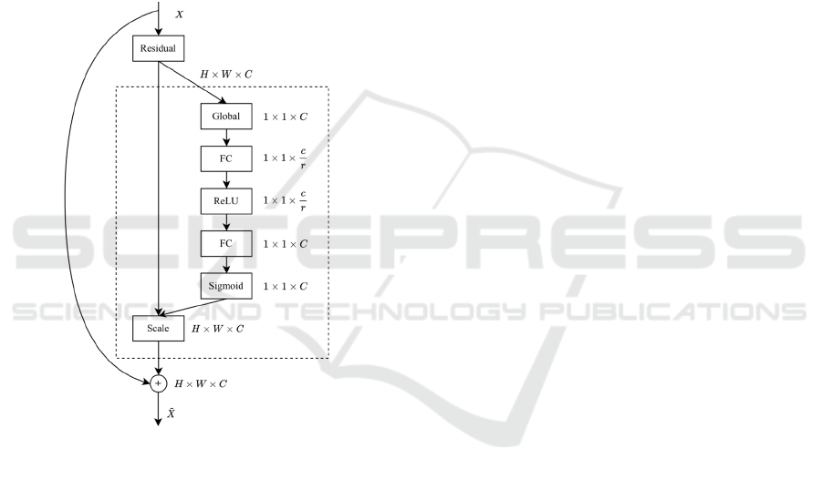
Figure 1: Resnet and SE-ResNet Block Structure.
While the SENet can be integrated into Resnet so
that we can get deeper SE-ResNet for our task. The
SENet ranked as the best performance in the ILSVRC
2017 image classification competition (Hu, Shen et
al. 2018). Besides investigating the spatial structure
of CNN, the SENet strengthened its learning
capabilities by using the relation among channels. Se-
Block is the core structure of the SENet. See the
dashed rectangle in Figure 1. The first step squeezes
the global spatial information into a channel
descriptor using global pooling. In the second step, a
gating mechanism is carried out on the descriptor
aiming at the limitation and generalization of the
model, which comprises three units, a full connection
layer for reducing the dimension, a ReLU, and a full
connection layer for increasing the dimension. A
sigmoid function is employed in the third step to
extract the channel-wised dependencies. Finally, this
dependency information is rescaled to the input
channels.
In CNN, channels represent the feature maps, i.e.,
the different levels of learned features. With more
layers, more features should be learned from the
network. The integrated features would be more
beneficial because some features would take effect
under some circumstances, and others would do
under other circumstances. Intuitively, can the
network learn the different importance of features to
take effect automatically when it is helpful for the
SVD?
As discussed, the SENet could answer this
question by modelling the channel relation. That is
why we employed SE-ResNet in this paper.
To conclude, we would like to employ Resnet
with various depths to extract the different levels of
features and then use Se-Block to choose the suitable
features to discriminate between the voice and the
non-voice segment.
3.2 Input Feature
As discussed, we computed only the kind of essential
feature, LMS, as the input. Ordinarily, the original
music signal was resampled at 22050Hz, and then we
calculated the spectrogram. After applying the Mel
scale to the spectrogram, we made the amplitude
logarithmic. We cut off the frequency band from 27.5
Hz to 8kHz. The frame length was 1024, and the hop
size was 315, i.e., 14.3ms. We segmented the LMS
feature into the 80 80 images and then fed them
into the SE-ResNet, with the hop size 5. So, the total
hop size was 71.5ms, and every image length was
1144ms.
3.3 SE-ResNet with Various Depth
To find the suitable depth for the task, we designed
the SE-ResNet with the depths 14, 18, 34, 50,
101,152, and 200, of which the majorities were by the
typical depths of Resets (He, Zhang et al. 2016),
except the first and last one. The networks with
depths 18 and 34 were piled up with the basic block,
while the bottleneck block was for depths 50, 101,
and 152 (He, Zhang et al. 2016). The SE-Blocks were
embedded into the primary or bottleneck block to
recalibrate the channel-wised weight. As examples,
we demonstrate three different layers of network
structure in Table 1.
Since the input size is 80 80, the output image
sizes are 40, 20, 10, 5, and 3, respectively. The lines
ISAIC 2022 - International Symposium on Automation, Information and Computing
338
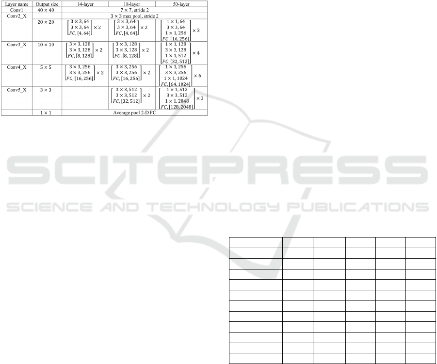
“FC” represent SE-Blocks, where the reduction
parameter was 16. The block scale parameters of the
34-layer, 101-layer, and 152-layer network are [3, 4,
6, 3], [3, 4, 23, 3], and [3, 8, 36, 3]. We added depths
14 and 200 in case the best performance would exist
on them. For the 14-layer network, we just modified
the 18-layer network by deleting the last layer. For the
200-layer network, the block scale parameter is [3,
12, 48, 3].
Table 1: SE-ResNet structure examples.
3.4 Training Configuration
We implemented the network on the PyTorch
framework with the help of the Homura package. We
employed the step-wise learning rate scheduler with
step size 10. The cross-entropy was used as the loss
function, and Adam was the optimizer with the
weight decay 110
. We also had the early
stopping mechanism, and the patience was set to 5.
We usually could reach the early stopping around ten
epochs from the experiments, although we set the
maximum epoch as 100.
4 EXPERIMENTS AND RESULTS
This section presents experiments and results based
on SE-ResNet, showing better performance on public
datasets.
4.1 Datasets
We chose three publicly available datasets for
experiments. The first dataset is the Jamendo corpus
(JMD), which contains 93 songs with 371 minutes of
total length. The second is the RWC pop, which
contains 100 songs with 407 minutes of total length.
The third is the Mir1k. Relatively minor, it contains
133 minutes of total length and 1000 song clips with
durations ranging from 4 to 13 seconds.
We kept the original division of train, validation,
and test datasets for JMD (Leglaive et al., 2015; Lee
et al., 2018; Lehner et al., 2018) unchanged, i.e., 61
songs for train, 16 for validation, and 16 for the test.
We divided the RWC dataset by which the songs
ending with the numbers 0-4 were picked up as the
training dataset, 5 and 6 as the validation dataset, and
7-9 as the test dataset. We separated the Mir1k
datasets by which the songs starting with a-g were
chosen as the parts for the training dataset, h-k
(including K) as the validation dataset, and l-z as the
test dataset.
Finally, we combined all three datasets into a
whole dataset by integrating the corresponding
training, validation, and test datasets. Hence, we got
a new dataset called the JRM dataset.
4.2 Comparison of Results
In this paper, we compare the performances based on
the pure models without data augmentation and other
processing, such as HPSS (Lee et al., 2018). Since the
state-of-the-art performances are conducted by
SCNN and RNN (Lee et al., 2018; Lehner et al.,
2018), we designed the experiments to compare our
algorithm and theirs. To some extent, it is fair to
demonstrate the capabilities of the networks in this
way.
Table 2: Network Performances on datasets. The Avg
denotes the average accuracy on RWC, Mir1k, and JMD.
The bold accuracies are the best of SE-ResNets (SERN is
the abbreviation in the table) on the same datasets.
RWC Mir1k JMD Avg JRM
SCNN 0.879 0.876 0.868 0.874 0.873
Bi-LSTM 0.875 0.865 0.875 0.872 0.878
SERN-14 0.899 0.880 0.890 0.890 0.890
SERN-18 0.895 0.882 0.877 0.885 0.890
SERN-34 0.891 0.881 0.897 0.890 0.891
SERN-50 0.912 0.869 0.877 0.886 0.899
SERN-101 0.910 0.870 0.846 0.875 0.897
SERN-152 0.901 0.880 0.885 0.888 0.901
SERN-200 0.900 0.873 0.881 0.884 0.887
LSTM Gain 0.025 0.015 0.01 0.016 0.022
SCNN Gain 0.022 0.004 0.017 0.014 0.027
In (Lee et al., 2018), as a third-party evaluation,
SCNN and Bi-LSTMs-based methods were
developed for revisiting. For SCNN, it only fed the
LMS feature, just the same as our approach.
Therefore, we directly used their results on Jamendo.
To obtain the results of SCNN on the databases RWC,
Mir1k, and JRM, we just run the train and test
programs on the respective datasets. For Bi-LSTMs,
we have tried two versions. One was done without
Singing Voice Detection Based on a Deeper Convolutional Neural Network
339
HPSS, and the other with HPSS as the original
version did. However, the performances without
HPSS were always worse than their counterparts from
experiments. For example, the accuracy was only
0.8003 on JRM. Hence, we did not put it on the table.
On the other hand, we run our algorithm
implementation on the datasets with various depths to
get the performances. We show all the results in terms
of accuracy in Table 2.
From the results, if we used the SE-ResNet with a
depth of 152, the improvement for SCNN and Bi-
LSTM would be on the “SCNN Gain” and “LSTM
Gain” lines, respectively. On the more
comprehensive dataset JRM, which is more
convincing, the accuracies are improved by 2.73%
and 2.29%, respectively. The best performance on
JMD is better than the state-of-the-art method, in
which the five different features were concatenated to
feed to the RNN.
4.3 Results of SE-ResNet with Different
Depths
Due to the amount and diversity of the data for
different datasets, the different depths would lead to
different performances. We show the results in terms
of accuracy on the four mentioned datasets with the
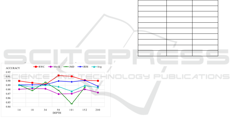
different depths of SE-ResNet in Figure 2.
Figure 2: Accuracy with different depths of SE-ResNet.
The performance on the combined dataset JRM
reaches the highest accuracy of 0.9012 at the depth
152, whereas the others reach the peaks at the mid-
depths (50, 18, 34) on (RWC, Mir1k, Jamendo). It
proves that if there is enough data, the deeper SE-
ResNet would be more potential to get better
performance. Otherwise, the best performance could
end with relatively shallower networks. The deeper
networks tend to be overfitting on the small datasets,
so they cannot obtain the best performance.
It is also worthwhile to note that the performance
on JRM is better than the Avg line. It means the
combination of the three fundamental datasets can
strengthen the overall learning capability of the
network.
4.4 Computation Cost
The network determines the number of parameters
(NoP). Although the Bi-LSTM has the minimum
NoP, it consumes the maximum CC. At the same
time, the computation cost (CC) depends on many
factors, such as the network scale, the network
converging mechanism, and the implementation
method. We ran the programs on the TITAN XP with
12G memory and evaluated CC by minutes per
training, including validation epoch on dataset JRM.
Table 3:
NoP
and CC of the networks on JRM. SERN is
the abbreviation for
SE-ResNet
in the table.
Networ
k
NoP (M) CC (min)
SCNN 1.4 7
Bi-LSTM 0.1 97
SERN-14 2.8 8
SERN-18 11 10
SERN-34 21 14
SERN-50 26 18
SERN-101 47 24
SERN-152 65 29
SERN-200 118 41
5 CONCLUSIONS
In this study, we proposed a novel SVD algorithm
based on SE-ResNet, which can be very deep.
Furthermore, we investigated the effect of the
different depths of SE-ResNet on the datasets. If we
had a more comprehensive and significant data
dataset, the deeper the network, the better the
performance. The experimental results demonstrated
that we obtained better results than published
systems.
ACKNOWLEDGEMENTS
This research was funded by the Major Program of
Natural Science Foundation for Jiangsu Higher
Education Institutions of China, grant number
22KJA520001, by the Jiangsu Overseas Visiting
Scholar Program for University Prominent Young &
Middle-aged Teachers and Presidents, and by the
Jiangsu Province Modern Education Technology
Research Project, grant number 2022-R-105945.
ISAIC 2022 - International Symposium on Automation, Information and Computing
340

REFERENCES
Berenzweig, A. L., & Ellis, D. P. (2001). Locating singing
voice segments within music signals. In Proceedings of
the 2001 IEEE Workshop on the Applications of Signal
Processing to Audio and Acoustics (WASPAA), pp.
119–122. IEEE.
Gupta, C., Yilmaz, E., & Li, H. (2020). Automatic lyrics
alignment and transcription in polyphonic music: does
background music help? In ICASSP 2020 - 2020 IEEE
International Conference on Acoustics, Speech and
Signal Processing (ICASSP), pp. 496–500. IEEE.
He, K., Zhang, X., Ren, S., & Sun, J. (2016). Deep residual
learning for image recognition. In Proceedings of the
IEEE Conference on Computer Vision and Pattern
Recognition (CVPR), pp. 770–778. IEEE.
Hsieh, T., Cheng, K., Fan, Z., Yang, Y., & Yang, Y. (2020).
Addressing the confounds of accompaniments in singer
identification. In ICASSP 2020-2020 IEEE
International Conference on Acoustics, Speech and
Signal Processing (ICASSP), pp. 1–5. IEEE.
Hu, J., Shen, L., & Sun, G. (2018). Squeeze-and-excitation
networks. In Proceedings of the IEEE Conference on
Computer Vision and Pattern Recognition (CVPR), pp.
7132–7141. IEEE.
Huang, H. M., Chen, W. K., Liu, C. H., & You, S. D.
(2018). Singing voice detection based on convolutional
neural networks. In 2018 7
th
International Symposium
on Next Generation Electronics (ISNE), pp. 1–4. IEEE.
Krause, M., Müller, M., & Weiß, C. (2021). Singing voice
detection in opera recordings: a case study on
robustness and generalization. Electronics, 10(10),
1214. MDPI.
Lee, K., Choi, K., & Nam, J. (2018). Revisiting singing
voice detection: a quantitative review and the future
outlook. In Proceedings of the 19
th
International
Society for Music Information Retrieval Conference
(ISMIR), pp. 506–513. Elsevier.
Leglaive, S., Hennequin, R., & Badeau, R. (2015). Singing
voice detection with deep recurrent neural networks. In
IEEE International Conference on Acoustics, Speech
and Signal Processing (ICASSP), pp. 121–125. IEEE.
Lehner, B., Schlüter, J., & Widmer, G. (2018). Online,
loudness-invariant vocal detection in mixed music
signals. In IEEE/ACM Transactions on Audio, Speech,
and Language Processing, 26(8), pp. 1369 – 1380.
IEEE.
Lin, L., Kong, Q., Jiang, J., & Xia, G. (2021). A unified
model for zero-shot music source separation,
transcription and synthesis. In Proceedings of 22
nd
International Conference on Music Information
Retrieval (ISMIR). Elsevier.
Nobutaka, O., Kenichi, M., Jonathan, L. R., Hirokazu, K.,
& Shigeki, S. (2008). Separation of a monaural audio
signal into harmonic/percussive components by
complementary diffusion on spectrogram. In 16
th
European Signal Processing Conference (EUSIPCO),
pp. 1–4. IEEE.
Rocamora, M., & Herrera, P. (2007). Comparing audio
descriptors for singing voice detection in music audio
files. In Proceedings of 11
th
Brazilian Symposium on
Computer Music, pp. 187–196.
Schlüter, J. (2016). Learning to pinpoint singing voice from
weakly labeled examples. In International Society for
Music Information Retrieval (ISMIR), pp. 44 – 50.
Elsevier.
Schlüter, J., & Grill, T. (2015). Exploring data
augmentation for improved singing voice detection
with neural networks. In International Society for
Music Information Retrieval (ISMIR), pp.121 – 126.
Elsevier.
Simonyan, K., & Zisserman, A. (2014). Very deep
convolutional networks for large-scale image
recognition. arXiv preprint arXiv:1704.02216.
Szegedy, C., Liu, W., Jia, Y., Sermanet, P., Reed, S.,
Anguelov, D., Erhan, D., Vanhoucke, V., &
Rabinovich, A. (2015). Going deeper with
convolutions. In Proceedings of the IEEE Conference
on Computer Vision and Pattern Recognition (CVPR),
pp. 1–9. IEEE.
Voigtlaender, P., Krause, M., Osep, A., Luiten, J., Sekar, B.
B. G., Geiger, A., & Leibe, B. (2019). MOTS: Multi-
object tracking and segmentation. In Proceedings of the
IEEE/CVF Conference on Computer Vision and
Pattern Recognition (CVPR), pp. 7942–7951. IEEE.
Zeiler, M. D., & Fergus, R. (2014). Visualizing and
understanding convolutional networks. In European
Conference on Computer Vision (ECCV), pp. 818–833.
Springer.
Zhao, S., Li, Q., He, T., & Wen, J. (2022). A step-by-step
gradient penalty with similarity calculation for text
summary generation. Neural Processing Letters, 1–16.
Zhao, S., Liang, Z., Wen, J., & Chen, J. (2022). Sparsing
and smoothing for the seq2seq Models. IEEE
Transactions on Artificial Intelligence, 1–10.
Zhao, S., Zhang, T., Hu, M., Chang, W., & You, F. (2022).
AP-BERT: Enhanced pre-trained model through
average pooling. Applied Intelligence, 52(14), 15929–
15937.
Singing Voice Detection Based on a Deeper Convolutional Neural Network
341
