
Semi-Autogenous Grinding Mill (SAG) Overload Forecasting Using
Gram Penalized Matrices in a CNN
R. Hermosilla
1 a
, H. Allende
1 b
and C. Valle
2 c
1
Universidad T
´
ecnica Federico Santa Mar
´
ıa, Valpara
´
ıso, Chile
2
Universidad de Playa Ancha de Ciencias de la Educaci
´
on, Chile
Keywords:
Overload Forecasting, SAG Mill Overload, Multivariate Times-Series Forecasting, Image Encoding for
Time-Series, Time-Series CNN, CNN Explanation.
Abstract:
In mining, detecting overload conditions is an opportunity to perform SAG mill to optimal operating condi-
tions. With this in mind, several authors have prove using machine learning mechanisms to detect overloads.
Our proposal establishes and tests a series of techniques to detect and forecast these events. Finally, we will
look for an explanation of what the model considers for classification improving the phenomenon knowledge.
Inspired by previous work and how operators classify overloads by analyzing behavior graphs of the most
relevant variables, we proposed a framework that includes selection, encoding, and filtering improvement to
finally discover the importance of the characteristics observed by our model using explanation techniques.
Thus, using a group of novelty techniques, our advances exceed the results presented by other authors and by
ourselves in previous publications, opening the door to a model based on attention in the future.
1 INTRODUCTION
In the mining context, comminution is the process that
reduces the ore size. In the case of most Chilean min-
ing, to obtain smaller particles for the next step in the
copper extraction (flotation).
Usually, this process includes crushing and grind-
ing equipment in a circuit composed of several stages.
SAG mill (semi-autogenous grinding) can process
large amounts of ore in the so-called primary grind-
ing stage. Usually, this process includes crushing and
grinding equipment in a circuit composed of several
steps. The efficient use of SAG mills means an in-
crease in ore production.
A 1% increase in SAG mill treatment supposes
a profit increase of up to US$160 MM per year and
between 200 and 400 tons of CO
2
emissions saving
under the same electricity consumption (Wakefield
et al., 2018; Pontt et al., 2012; Northey et al., 2013).
However, achieving these efficiency levels has the
risk of overload, a condition that limits the opera-
tion. Divers authors have tried to identify through
several techniques such as the theoretical analysis
a
https://orcid.org/0000-0002-6032-4811
b
https://orcid.org/0000-0002-9899-0051
c
https://orcid.org/0000-0001-7158-2069
of variables (Strohmayr and Valery, 2001; Powell
et al., 2009), use of predictive control ((Forbes and
Gough, 2003)), making simulation models (Varas
et al., 2019), through linear programming (C
´
esar and
Daniel, 2009) or using machine learning techniques
(Ko and Shang, 2011; McClure and Gopaluni, 2015;
Hermosilla et al., 2021).
In our research, we have established a mechanism
that allows the classification and early detection (fore-
cast) of overloads as a multivariate binary classifica-
tion model.
Inspired by the work performed in the generation
of encodings based on distance matrices (Bardinas
et al., 2018) and the analysis that expert metallur-
gists to determine the occurrence of overloads, we
have proposed a deep convolutional neural network
that uses the feature relationship using a multivariate
approach of Gram’s matrix as an encoder.
In other words, we proposed the generation of ma-
trices with angular differences of the feature pair ar-
rays as input for our model. Those matrices are penal-
ized with a temporary degradation filter that penalizes
the oldest data, trying to establish a mechanism for
differentiating the temporal data used in each encoded
time window, which has yielded promising results.
Finally, we uncover, through explanation mecha-
nisms, the combinations of variables/time that most
Hermosilla, R., Allende, H. and Valle, C.
Semi-Autogenous Grinding Mill (SAG) Overload Forecasting Using Gram Penalized Matrices in a CNN.
DOI: 10.5220/0011946800003612
In Proceedings of the 3rd International Symposium on Automation, Information and Computing (ISAIC 2022), pages 391-396
ISBN: 978-989-758-622-4; ISSN: 2975-9463
Copyright
c
2023 by SCITEPRESS – Science and Technology Publications, Lda. Under CC license (CC BY-NC-ND 4.0)
391

affect the prediction of overloads.
The following chapters explain the overload phe-
nomenon and how we have approached a solution.
Section 2 explains the overload phenomenon and its
importance in the comminution process. Section 3
will delve into our proposal and how we address it
through a set of proposed methods. Section 4 shows
our results. Section 5 shows our conclusions and fu-
ture work.
2 OVERLOAD DETECTION AND
RELATED WORK
Maximizing ore treatment is one of the main goals of
a SAG mill operation. Though, this objective depends
on several factors that can influence the occurrence of
an overload event.
Factors such as the distribution of solids, hardness,
excessive load volume, particle size distribution, the
number of steel balls, and wear, among others, can
generate an overload condition.
2.1 Overload Types
In a SAG mill can found three kinds of overloads can
occur (Fig. 1).
In all cases of overload, mill loses the cataract
4
property generating a vicious circle that leads to
the ineffectiveness of the equipment. The volumetric
overload occurs when the SAG mill is overfed. Ore’s
hardness, size, or composition can produce this con-
dition.
When excess water attenuates the fall’s effect, it
is declared an overload by slurry pooling, affecting
the ore’s size reduction, producing accumulation and
next, a volumetric overload. When the pulp covers
the lifters, a freewheeling overload is declared. The
pulp on the lifters avoids the ore rising, inhibiting the
cascade.
Also, composition, distribution, and load fill can
influence an overload occurrence. We can search this
behavior by observing the power consumed but only
at the beginning of an overload (Apelt et al., 2001),
without enough foreseeing.
The distinct factors and the complex relations of
the features underlying the overload make obtaining a
physical forecast overload system hard. However, es-
tablishing a model based on data that learn this com-
plex relationship is possible. Thus, our research fo-
cused on obtaining an overload forecast model based
4
Ore rises to the top of the mill, breaking on the impact
zone.
Figure 1: SAG mill overloads.
on a time-series classification with a multivariate ap-
proach.
2.2 Related Work
According to our research, two approaches exist at
least to address the SAG mills’ overloads and under-
stand the problems associated with their operation.
One seeks to generate an adequate operation from
the control point of view, and the other focuses on
seeking the occurrence of overloads.
Among these investigations, ((Salazar et al.,
2014)) establish a control and prediction mechanism
for the behavior of the mill using a method called
Multiple Input/Multiple Output Predictive Control
Model (MIMO MPC).
The authors prove the relationship between the op-
erating variables based on load tonnage.
His work also allowed the establishment of simu-
lated operating conditions of an overload state, keep-
ing the controlled variables without relevant variation.
On the other hand, (Wang et al., 2020) allowed to
establish overload-free operating conditions through
the control of the speed of the mill, generating an op-
timal operating space describing the relationship be-
tween speed, ore quantity, and particle size.
However, one of the nearest research to our line of
study is published by (McClure and Gopaluni, 2015),
which experiments with techniques like KPCS, SVM,
and LLE to classify overloads (not predict them).
Likewise, our previously published research ad-
vanced toward constructing an overload prediction
framework using deep networks.
Now, we have improved results by better under-
standing the underlying phenomenon and the inclu-
ISAIC 2022 - International Symposium on Automation, Information and Computing
392

sion of elements, such as the degradation or penalty
filter.
In the previous work, we intuited could be ex-
plained the network in some way.
In this proposal, we have included a way to ex-
plain the network and analyze the results, allowing
contrasting the model’s decisions with experts’ opin-
ions.
3 OVERLOAD FORECASTING
PROPOSED METHOD
As we have pointed out, we propose approaching our
overload prediction problem through a multivariate
binary classification model based on deep convolu-
tional neural networks.
So, we have to overcome several difficulties, such
as adequately selecting operation variables, generat-
ing a representative encode, or attending a highly un-
balanced scenario (less than 2% of the labeled data
corresponds to overloads).
Furthermore, we will add a filter that has given us
promising results penalizing past data and the applica-
tion of an interpretation method called Grad-CAM++
(Chattopadhay et al., 2018) to determine and check
the dependency of the selected relationships with our
target.
3.1 Base Definition
Let y = [y
1
, . . . , t
′
]
T
with T ∈ [1, . . . , T
′
] as the set
of values binaries that describe the overload condi-
tion every time t t (y
t
= 1 as an overload at time
t). We will assume the matrix T
′
× N as the matrix
X = [x
1
|. . . |x
T
′
]
T
that expresses the collection of vec-
tors x
t
formed by the N available and selected fea-
tures. That is, x
( j)
t
denotes the value of the j − th
characteristic at time t.
Expressed our approach as a multivariate time-
series problem that symbolizes a stochastic process,
we define our goal as overload forecasting y
t+k
, thus,
in k steps ahead of the current observation t. Given
that the associated distribution of the underlying pro-
cess is unknown, we assume our model will learn the
relationship of values observed previously to forecast
the overload occurrences. Then, we modeled the val-
ues’ fit as p(y
t+k
|x
t
, ..., x
t−w−1
) in w steps to the past.
3.2 Feature Selection by Pairs
We propose to train a deep convolution neural net-
work to learn the relationship of the available features
through a structure that includes pairing the variables
with the highest relationship with the overload.
Inspired by the classification of overloads
achieved by metallurgical experts, we intend to select
those pairs that provide the most information regard-
ing our target.
We solved this using Conditional Mutual Informa-
tion (CMI) (Liang et al., 2019) to get a reduced num-
ber of pairwise relations, looking for pairs related to
adding the maximum information possible about our
target. We express CMI as follows:
I(x
(i)
, x
( j)
|y) = E
y
[D
kl
(P
(x
(i)
,x
( j)
|y)
||P
(x
(i)
|y)
⊗P
(x
( j)
|y)
)],
(1)
where I(x
(i)
, x
( j)
|y) is the value expected respect to y,
of the relative entropy or Kullback-Leibler divergence
D
kl
from conditional joint distribution P
(x
(i)
,x
( j)
|y)
to
the product ⊗ of conditional marginals P
(x
(i)
|y)
and
P
(x
( j)
|y)
.
Accordilyng, let define z
r
= (z
(1)
r
, z
(2)
r
) as a matrix
with features pairs x
(i)
and x
( j)
selected from rth bet-
ter CMI values (1).
Let z
r
= (z
(1)
r
, z
(2)
r
) as a matrix with features pairs
x
(i)
and x
( j)
selected from rth better CMI values (1).
Let
˜
Z as an array with three dimensions w × w ×
R, with window length w and the number of selected
pairs R, each composed by ˜z
(i)
tr
.
3.3 Encoder by Matrices Inspired in
Gram
Problems such as univariate time series have recently
been solved using gram matrices (Wang et al., 2022);
however, we will use it as a multivariate approach ap-
plying some changes. After selecting R pairs on top of
CMI ranking time series X using the technique min-
max scaler, we transform each pair z
1
, . . . , z
R
to the
space [−1, 1] as follow:
˜z
(i)
tr
=
z
(i)
tr
− min(z
(i)
r
)
max(z
(i)
r
) − min(z
(i)
r
)
, i = 1, 2, t = 1,
. . . , T, r = 1, . . . , R,
(2)
where minimum value min(z
(i)
r
) and maximum value
max(z
(i)
r
) of the ith selected feature.
Then, we transform ˜z
(i)
tr
to polar coordinates throw
the cosine of the angle of the values, and obtaining the
radius ρ using the timestamp ts
t
, given by:
Semi-Autogenous Grinding Mill (SAG) Overload Forecasting Using Gram Penalized Matrices in a CNN
393
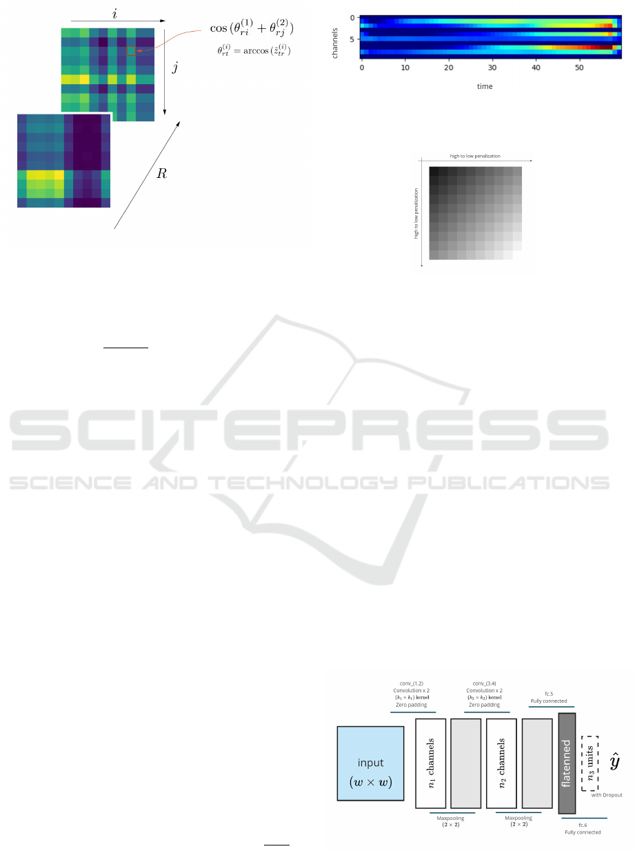
Figure 2: Image generated with GADF approach with R
pairs/channels.
θ
(i)
rt
= arccos(˜z
(i)
tr
), −1 ≤ ˜z
(i)
tr
≤ 1, (3)
ρ
t
=
ts
t
max(ts)
, ts
t
∈ ts,
where the value of the timestamp is represented by ts
t
,
and the maximum value of all timestamps is wrote as
max(ts).
The next step in our process is to apply a Gramian
approach to the angle differences of each pair to ob-
tain a three-dimensional array G with w × w × R di-
mensions. Here, g
r(i, j)
represents each pixel in posi-
tion (i, j) of rth Gram’s matrix of G, as follows:
g
r(i, j)
= cos(θ
(1)
ri
+ θ
(2)
r j
), i, j = 0, . . . , w − 1,(4)
where θ
(1)
ri
and θ
(2)
r j
represents the transformed pair se-
lected previously. We can understand G as the render-
ing of an image with R channels, where each image
represents the angular variation of the top-R CMI’s
ranking selected pairs (Figure 2).
3.4 Penalization over Time
Sub-Matrices
As we can guess, overloads are a phenomenon that
increases as we get closer to the moment of their ap-
pearance. Also, after making our models, we verified,
using an explanation method (4.2), that in the cases
in which overloads occur, our model considered the
instants prior to the evaluated time to be more critical
(Figure 3). Based on these antecedents, we define a
filter that allows us to penalize those previous values
in each channel of the encoder.
Let f = [0, . . . , w − 1] define the filter F =
f + f
T
2w
,
which will generate a filter of dimension w × w with
Figure 3: Importance by selected pairs over overload clas-
sification. Blue and red colors represent low and high im-
portance, respectively.
Figure 4: Filter applied in each channel.
values in R in the interval [0, 1] which we will ap-
ply to each of the channels R of the generated images
G (Figure 4). As we will see in chapter 4, this sim-
ple method allowed us to improve our model signifi-
cantly.
3.5 Convolutional Neural Network
The set of images G are taken by a deep convolutional
neural network (Fig. 5), made up of convolutional
layers with n
1
filters of k
1
× k
1
size and 2 × 2 max-
pooling, followed by a batch normalization layer.
We added once more time the same set of convo-
lutional, max-pooling and batch normalization layers
(with the same hyperparameters). All the convolu-
tional layers have ReLU as an activation function and
zero padding.
Finally, the last layer is fully connected with a flat-
ter layer, followed by n
3
nodes with Dropout dense
layer, to end with one single neuron as output for bi-
nary classification using a sigmoidal activation func-
tion. Due to the highly imbalanced scenario found,
Figure 5: Convolutional Neural Network Architecture.
ISAIC 2022 - International Symposium on Automation, Information and Computing
394

we use focal binary crossentropy as a cost function
setting with class weights parameters.
4 EXPERIMENTS AND RESULTS
Obtaining a forecast with ten minutes of anticipation
is our primary goal. Considering a 30 seconds resolu-
tion, we set k = 20 in our target y
t
+k. Also, we define
w = 60 as the offset into the past, ergo 30 minutes.
We have a dataset with around 700k labeled
records strongly imbalanced (1.46% imbalanced ra-
tio), corresponding to nearly twelve months of data.
We selected 48 of 72 features linearly indepen-
dent. With these 48 features we start our process
of selecting the K = 10 top pairs corresponding to
{( f in, gru), (pot, dm ), (ton, dm ), ( f in, int), (gru, int),
(pre, vel), (pot, vel), (pot, pre), (pre, dm ), (int, pre)}
5
.
After selecting our top feauture pairs, we build the
G matrices using our Gram’s matrices approach. Due
to time-missing values, this process reduced the num-
ber of matrices to around 685k, reducing our imbal-
anced ratio to 1.38%.
We setted the network hyperparameters with n
1
=
256, n
2
= 128, n
3
= 512 nodes for each layer using the
grid search method. Using the same way we setted
(k
1
× k
1
) = (k
2
× k
2
) = (3 × 3) for the kernels size.
We setted the optimizer as Adam with learning rate
(lr = 0.001).
To train we use a cross-validation technique pro-
posed by (Bergmeir and Ben
´
ıtez, 2012) for time se-
ries.
4.1 Evaluation Methods
Table 1 shows the average sensitivity, specificity, and
F1 score with the respective standard deviation to the
model based on LLE+LDA as suggested by (McClure
and Gopaluni, 2015), we have also included the re-
sults of our previously proposed model (Hermosilla
et al., 2021), and the results of this proposal, without
filter (⋆) and with penalization filter. As can be seen,
the proposed model with the applied filter exceeded
the previous results significantly.
4.2 GradCAM++ CNN Explanation
The authors (Chattopadhay et al., 2018) proposed a
generalized method called Grad-CAM++ that is for-
mulated by explicitly modeling the contribution of
5
fin: fine granulometry, gru: coarse granulometry, dm :
milliseconds from the last maintenance, int: intermediate
granulometry, pre: pressure, vel: velocity, ton: total ton-
nage.
Figure 6: Example of cluster generated with a explanation
model based on GradCam++.
each pixel in the feature maps of a CNN to the fi-
nal output. With this, it is possible to look at the el-
ements to which the network pays attention in each
case. To do this, they reformulate the structure of the
w
k
c
weight for c class in k layer of the network:
w
k
c
=
∑
i
∑
j
α
kc
i j
.relu
∂Y
c
∂A
k
i j
!
, (5)
where relu is the Rectified Linear Unit activation
function, α
kc
i j
are the weights of the gradients for a
particular pixel i, j, and Y
c
are the values of the partic-
ular class to analyze. w
k
c
will capture the importance
of the activation map A
k
.
Using this method, we characterized the overloads
to understand feature pairs directly influencing the
target. Have been clustered the results to achieve
an analysis of the leading classification groups of the
model.
In Figure 6, we can see an example of how the
model considers the pairs of channels 5, 6, 8, and 9
most relevant in the periods close to the overload oc-
currence.
Precisely channels 5 ({pre}, {vel}) and 6 ({pot},
{vel}) are relationships, which experts use to clas-
sify overloads. However, channels 8 and 9, with pairs
(pre, dm ), (int, pre), seem particularly relevant to the
model and offer an opportunity to use new relations to
the study of overload genesis.
An interesting observation is that even having pe-
nalized the times far from the moment t, in all cases,
the model highlights those instants as essential for the
classification, which makes us suppose that the infor-
mation contained in the first moments of the charac-
teristics matrix G is essential for forecasting.
Semi-Autogenous Grinding Mill (SAG) Overload Forecasting Using Gram Penalized Matrices in a CNN
395

Table 1: Average and standard deviation over S test sets.
Model Sensitivity Specificity F1
LLE+LDA 0.555(±0.425) 0.453(±0.321) 0.440(±0.298)
Previous proposed model 0.643(±0.227) 0.894(±0.106) 0.609(±0.084)
Proposed model⋆ 0.653(±0.124) 0.889(±0.178) 0.742(±0.098)
Proposed model 0.871(±0.134) 0.838(±0.102) 0.859(±0.113)
5 CONCLUSIONS AND FUTURE
WORKS
In this work, we propose improving the methods to
arrive at an overload forecasting model in a complex,
multivariate, and highly unbalanced problem using a
Gram matrix-based encoding.
We take advantage of the benefits of the CNNs to
generate a model that allows us to know the relation-
ships of these matrices with the overload.
The experimental results show that we have over-
come the approach in previous works and state of the
art.
Using an explanation method called Grad-
CAM++, we established some interesting study sets
for expert review, for example, the relationship be-
tween pressure and timing of equipment maintenance
and fine grain size and pressure to explain some over-
loads.
Also, this behavior could allow us to increase the
forecast distance. In the future, we will integrate the
care information in the same network to generate a
model specialized mainly in those elements that most
influence the occurrence of overloads.
REFERENCES
Apelt, T., Asprey, S., and Thornhill, N. (2001). Inferential
measurement of sag mill parameters. Minerals engi-
neering, 14(6):575–591.
Bardinas, J., Aldrich, C., and Napier, L. (2018). Predict-
ing the operating states of grinding circuits by use of
recurrence texture analysis of time series data. Pro-
cesses, 6(2):17.
Bergmeir, C. and Ben
´
ıtez, J. M. (2012). On the use of cross-
validation for time series predictor evaluation. Infor-
mation Sciences, 191:192–213.
C
´
esar, G. Q. and Daniel, S. H. (2009). Multivariable model
predictive control of a simulated sag plant. IFAC Pro-
ceedings Volumes, 42(23):37–42.
Chattopadhay, A., Sarkar, A., Howlader, P., and Balasub-
ramanian, V. N. (2018). Grad-cam++: Generalized
gradient-based visual explanations for deep convolu-
tional networks. In 2018 IEEE winter conference on
applications of computer vision (WACV), pages 839–
847. IEEE.
Forbes, M. G. and Gough, B. (2003). Model predictive con-
trol of sag mills and flotation circuits.
Hermosilla, R., Valle, C., Allende, H., Lucic, E., and Es-
pinoza, P. (2021). Semi-autogeonous (sag) mill over-
load forecasting. In Iberoamerican Congress on Pat-
tern Recognition, pages 392–401. Springer.
Ko, Y.-D. and Shang, H. (2011). Sag mill system di-
agnosis using multivariate process variable analy-
sis. The Canadian Journal of Chemical Engineering,
89(6):1492–1501.
Liang, J., Hou, L., Luan, Z., and Huang, W. (2019). Feature
selection with conditional mutual information consid-
ering feature interaction. Symmetry, 11(7):858.
McClure, K. and Gopaluni, R. (2015). Overload de-
tection in semi-autogenous grinding: A nonlinear
process monitoring approach. IFAC-PapersOnLine,
48(8):960–965.
Northey, S., Haque, N., and Mudd, G. (2013). Using sus-
tainability reporting to assess the environmental foot-
print of copper mining. Journal of Cleaner Pro-
duction, 40:118–128. Special Volume: Sustainable
consumption and production for Asia: Sustainability
through green design and practice.
Pontt, J., Valderrama, W., Olivares, M., Rojas, F., Robles,
H., L’Huissiers, S., and Leiva, F. (2012). Uso eficiente
de la energia en procesos mineros. Centro de automa-
tizacion para la industria minera, Chile.
Powell, M., Van der Westhuizen, A., and Mainza, A. (2009).
Applying grindcurves to mill operation and optimisa-
tion. Minerals Engineering, 22(7-8):625–632.
Salazar, J.-L., Vald
´
es-Gonz
´
alez, H., Vyhmesiter, E., and
Cubillos, F. (2014). Model predictive control of semi-
autogenous mills (sag). Minerals Engineering, 64:92–
96.
Strohmayr, S. and Valery, W. (2001). Sag mill circuit op-
timisation at ernest henry mining. In Proceedings of
the SAG 2001 Conference, Vancouver, BC, Canada,
volume 30.
Varas, P., Carvajal, R., and Ag
¨
uero, J. C. (2019). State
estimation for sag mills utilizing a simplified model
with an alternative measurement. In 2019 IEEE
CHILEAN Conference on Electrical, Electronics En-
gineering, Information and Communication Technolo-
gies (CHILECON), pages 1–7. IEEE.
Wakefield, B., Lindner, B., McCoy, J., and Auret, L. (2018).
Monitoring of a simulated milling circuit: Fault diag-
nosis and economic impact. Minerals Engineering,
120:132–151.
Wang, J., Li, S., Ji, W., Jiang, T., and Song, B. (2022). A
t-cnn time series classification method based on gram
matrix. Scientific Reports, 12(1):1–14.
Wang, X., Yi, J., Zhou, Z., and Yang, C. (2020). Optimal
speed control for a semi-autogenous mill based on dis-
crete element method. Processes, 8(2):233.
ISAIC 2022 - International Symposium on Automation, Information and Computing
396
