
On Detection and Classification of State Changes in Physical
Processes by Signal Processing Techniques
Dorel Aiordachioaie
Department of Electronics and Telecommunications,
Dunarea de Jos University of Galati, Romania
Keywords: Signal Processing, Time-Frequency Transform, Image Processing, Information Processing, Source
Identification, Entropy, Feature Selection and Extraction.
Abstract: The paper presents a comparation of some methods based on signal processing, for detection and classification
of the changes in the states of physical processes. The investigated processes generate mechanical vibrations,
which are properly managed for computer-based processing. As a case study, the incipient faults in bearings
are considered. Five signal processing methods are promoted, which are based on statistical processing, signal
modelling, spectral analysis, time-frequency image processing, and information modelling. Statistical
processing method considers ten features based on statistical moments of various orders. The method of signal
modelling involves models with parameters estimated by an Kalman estimator. The method of spectral
analysis considers the power spectrum of the vibration’s signals. The method based on time-frequency
analysis considers the short-time Fourier transform and Choi-Williams transform for feature extraction. The
information-based method is based on information source identification and processing. The classifier is based
on similarity comparation using a distance-based classifiers. The novelty/contribution of the paper is the
evaluation of the methods for change detection and diagnosis, all based on signal processing paradigm. Each
of the considered method has advantages and disadvantages and depends on available data. The involved
techniques could be applied also in process monitoring and conditioning.
1 INTRODUCTION
In the operation of production processes, defects in
various elements of the components may occur. Their
incipient detection and limitation of interruptions in
production are of major importance in engineering
practice. Fault detection refers to such
problems/defects in the context of physical and – very
often – industrial processes. However, the use of this
expression may be limiting or inappropriate, as
possibly giving rise to mis interpretation in certain
cases. For example, changing the state of a variable
in the process can also be achieved without being
defective, by changing the regime and/or the load in
the process under study.
Change detection based on the recording and
processing of a single signal, in the simplest case, is
done by checking the "dynamic" range of the signal
(peak-peak value) or, in more complex cases, on the
extraction of features and the application of change
detection methods.
By detecting the change of a state is meant the
activity of sensing/ identifying the change of a state
(usually undesirable) in the operation of a system.
The processed signals are taken from the process or
are obtained from the use of a model, through
simulation. Such signals can be vibration signals,
sound waves of different frequencies (e.g., audio,
ultrasonic), and even electrical signals from the
investigated system
.
There are processes in which harmonic signals are
available (by measurements) and affected by a
greater or lesser number of noises, so they have a
random behavior. If the changes in these signals
correspond to defects in action elements, process or
sensors, methods based on signal-model-based can be
applied. A representative example is the vibration
monitoring application which allows, by measuring
position, speed or acceleration, the detection of non-
equilibrium or defective bearings.
An example of a complex process, in which the
detection of change and the detection of defects and
diagnosis are important activities are the case of a
440
Aiordachioaie, D.
On Detection and Classification of State Changes in Physical Processes by Signal Processing Techniques.
DOI: 10.5220/0011950800003612
In Proceedings of the 3rd International Symposium on Automation, Information and Computing (ISAIC 2022), pages 440-445
ISBN: 978-989-758-622-4; ISSN: 2975-9463
Copyright
c
2023 by SCITEPRESS – Science and Technology Publications, Lda. Under CC license (CC BY-NC-ND 4.0)

wind turbine, where faults can be in the mechanical
part (external blades, reducer box) or in the electrical
part (generator, converter, transformer, etc.). Another
case is of a rolling mill, where the mechanical part is
important in the quality of the product and is the part
dominated in the generation of defects, sources of
vibration signals, (Precup et al., 2015), (Seeliger et
al., 2002).
In the field of Change Detection and Diagnosis
(CDD) methods, two categories are important,
(Zhang & Jiang, 2008). The methods based on
model, process and/or measured signals, and methods
based on measured data. From the various available
methods, in this work it will be considered the
analytical method, based on the processing of the
vibration signals. Other examples and details are
available through the references (Isermann, 2006),
(Patton, et al, 1989), (Venkatasubramanian, et al,
2008), (Ypma, 2001), (Zhang, 2010).
The structure of the detection method by
analyzing the signal model assumes a mathematical
model for the signal, one can calculate specific
parameters such as: amplitudes, phases, frequency
spectra and correlation functions, for the frequency
of the signal. By comparison with the features
observed in normal function, analytical syndromes
are generated. Signal models can be parametric
(amplitudes for certain frequencies or specific type
models) or nonparametric (frequency spectra or
statistical correlation functions), (Iserman, 2006).
The detection of the changes by methods of
processing their signatures can be solved by several
methods, some of which are direct (i.e. the signal is
processed directly and the processed values have
physical significance) or indirect (values are
processed transformed into different spaces from the
original ones, where the processed data may or may
not have physical significance, (Timusk, et al, 2008).
In direct methods, the observed values are directly
calculated by calculating statistical quantities (most
often) or gradient-based criteria. These methods are
often applied in process monitoring applications by
processing vibrations and audio signals. The methods
are simple to understand and simple to implement,
sometimes with very good results, but less good in the
case of non-stationary signals or time-varying or
interdependent events (defects).
Indirect methods, based on transformations, are
more complex, but the calculations for decision
making in the new spaces of observations are simpler.
Compared to direct methods, indirect methods give
better results. The following types of transformations
can be exemplified here: time-frequency
transformations and entropic transformations (based
on the evolution of entropy).
The signals can be processed in the time domain,
in the frequency domain or in the combined/mixed
time-frequency domain. Each of these areas has
advantages and disadvantages, so a robust solution
involves a combination of methods from the fields
presented, (Popescu et al, 2017).
The paper is organized in five sections. The next
section presents the general structure of the methods
used for data processing and a short analysis of data
used in the testing stage. Section 3 presents the
principles of the promoted methods. Section 4
presents some results of the computer-based
experiments. Finnally, the conclusion section ends
the paper.
2 THE STRUCTURE OF THE
METHODS
The problem of change detection and classification of
faults in bearings is considered. The data used for
experiments are from (CWR, 2022). There are four
classes of signals, associated to four
states/cases/faults: F0- free of faults, F1- fault in ball,
F2 – fault in inner ring, and F4-fault in outer ring. For
each state/fault, a record of 200,000 samples is
available, which corresponds to an observation
interval of ten [s]. The motor speed is 1797 rpm, and
the working conditions are without mechanical load.
A test vector is considered with frames of 5,000
samples for each record, which is explored with a
sliding window of length w, variable from 100 to
5,000 samples, depending on the performance of the
detection. The bigger window the less precise is the
point change detection.
The structure of the data processing is presented
in Fig.1. Data are pre-processed by filtering and
scaling to [-1,1] interval. The next block computes the
features, and the classifier estimates the state/fault.
The input waveforms are quite similar, so the most
important block is the feature selector. A primary
frequency analysis shows an overlapping in
frequency domain, which will generate difficulties for
a right classification. This is a reason to explore more
than a method for CDD, as in the case of the present
paper, and to promote combination of methods from
the same domain or from different domains.
Figure 1: The structure of data processing.
On Detection and Classification of State Changes in Physical Processes by Signal Processing Techniques
441
3 THE METHODS
Five methods are considered for this work. Some are
used as references, e.g., statistical method, and others
are based on advanced processing techniques, as
those based on time-frequency techniques.
3.1 The Statistical Method
The basic theory and the computation of the statistical
moments are presented in (Gustafson, 2007),
(Shanmugan and Breipohl, 1988), and (Barkat, 2005).
Examples of the method under various simulation
scenarios are presented in (Basseville, 1997),
(Aiordachioaie, 2013).
Ten statistical features are used: the mean, the
dynamic range, the median, the variance, the mean of
the absolute values, the root mean squares, the peak
value, the crest factor, the skewness, and the kurtosis.
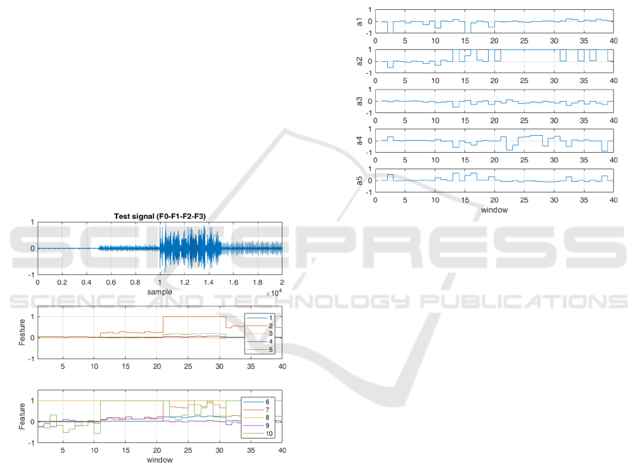
Fig. 2 presents the evolution of the feature set, for
an observation window with 500 samples. The
evolution of the features indicates the moment of
change. The process diagnosis depends on the
performance of the classifier.
Figure 2: Features of the statistical method.
3.2 The Signal Modelling Method
The principle of the method is to design an
autoregressive moving average (ARMA) signal
model, (Kay, 1993), (Poor, 1994), (Bozic, 2021) and
to estimate its parameters in each observation
window. A change in one or more parameters
indicates a change in the structure of the process.
The equation of the ARMA (Ma, Mb) model is
𝑦
𝑛
∑
𝑎
𝑛
𝑦
𝑛𝑘
∑
𝑏
𝑛
𝑣
𝑛
𝑗
𝑣
𝑛
(1)
where y(n) is the modelled signal, and v(n) is
Gaussian white noise. A Kalman estimator is used for
the estimation of the parameters, (Haykin, 2002).
Fig. 3 presents an example of the first five
parameters of the ARMA(5,5) model, during the test
with windows (of length 500 sample). More details of
the used method are available in (Aiordachioaie,
2014).
Figure 3: Features of the signal model-based method.
3.3 The Spectral Analysis Method
For each sliding data window, a power spectrum is
computed and analysed. The features vector is
composed of eight features: the mean and the
variance in frequency, the third and fourth order
centred statistical moments, the median, the energy in
frequency domain, and the mean and the variance
over the amplitude values. The basic equations are
presented in (Aiordachioaie, 2022a).
Fig. 4 presents the evolution of the feature set,
over a test vector composed of 40 windows. The
evolution allows the detection of the changes in the
test vector.
The method based on the features of power
spectra is called SF (Spectral Features) and the
method based on power spectra only is referred a SD
(Spectral Direct) in Table 1. In the case of SD method,
the spectral lines could be labelled as direct features.
The SD method needs a higher resolution than SF.
ISAIC 2022 - International Symposium on Automation, Information and Computing
442
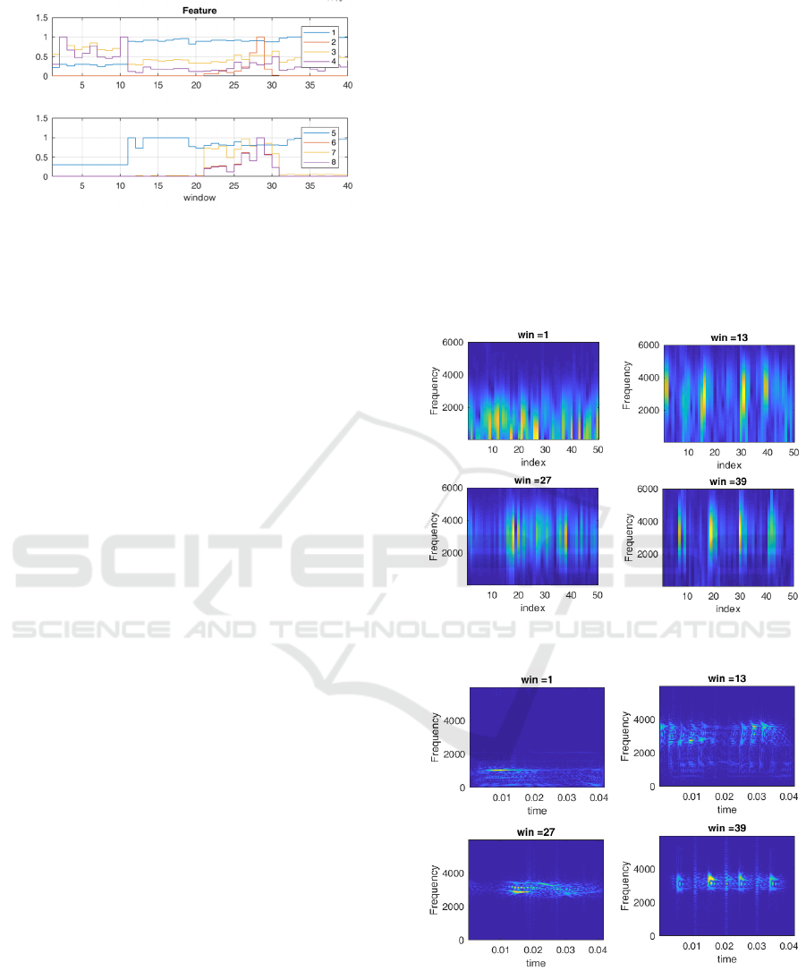
Figure 4: Evolution of the features in frequency domain.
3.4 Time-Frequency Analysis Method
The methods based on time-frequency transforms
(TFT) represent effective solutions for the detection
of change of in vibratory processes, since it is
detected the change in the frequency domain and the
moment of change in time domain, when they have
occurred. The approach is indicated for intermittent
and dynamic faults. Time-frequency analysis covers
a major area related to the non-stationary signals
(including transient ones) by the ability to detect and
to locate them.
Three most used methods are based on the short-
time Fourier transform (STFT), quadratic time-
frequency transform (e.g., Wigner transform) and
wavelet transform (WT). Some good references are
(Auger, 1991), (Boashash, et al, 2014), and (Cohen,
1989).
Let consider a signal x(t) and a sliding observation
window w(t). By discretization, a time-frequency
matrix is generated. The basic equations for the above
transforms are
𝑋
𝑛,
𝑓
∑
𝑥
𝑘
𝑤
𝑘𝑛
𝑒
(2)
for STFT, and
𝑊
𝑛,
𝑓
∑
𝑥
𝑘
𝑥
∗
𝑛𝑘
𝑒
(3)
for Wigner transform. In experiments, the Choi-
Williams transform (CWT) is used to decrease the
interference terms, (Barry, 1992), (Flandrin, et al,
1996). In the case of WT, the signal x(t) is
decomposed following the mother wavelet 𝜑, and the
coefficients a
lk
define the matrix of interest, (Mallat,
1989), and (Daubechies, 1992).
An efficient approach is to consider the
coefficients of the TFT as elements of a digital image,
and thus to obtain a time-frequency image (TFI).
Each observation window generates a TFI, which is a
matrix or a 2D signal.
Seven features are considered for an image as: the
mean, the variance, the skewness, the kurtosis, the
coefficient of variations, the spectral flux, the
frequency of the maximum amplitude. The
computation expressions are available in
(Aiordachioaie, 2022b).
Fig. 5 presents a set of TFI based on STFT. It is
about windows 1, 13, 27 and 39 from the set of 40.
On the x axis the index of the window is presented,
and on y axis the frequency in Hz. The size of the TFI
is 6001x50 pixel.
Fig. 6 shows a set of four TFI based on CWT for
the same set of windows. The time variable is
considered on the x axis. The size of the TFI is
500x500 pixel. This approach has a higher precision
referred to the previous one. By analysing and
classifying the content of the image, the change and
diagnosis could be easily solved.
Figure 5: Time-frequency images for STFT.
Figure 6: Time-frequency images for CWT.
The Fig.7 and 8 presents the evolution of some
features for the methods of time-frequency
approaches. A change in the signal is detected by one
or more changes of the selected features.
On Detection and Classification of State Changes in Physical Processes by Signal Processing Techniques
443

Figure 7: Feature evolution for STFT based method.
Figure 8: First four features for CWT based method.
3.5 The Information Processing
Method
Functions based on entropies is used for each data
window, e.g., Renyi entropy. A source identification
process is necessary before computation of the
entropies, to estimate the probabilities of the basic
elements. The approach can be applied directly to the
vibration signals (1D signals) or to time-frequency
images (2D signals) as in the present approach.
The set of the features has the Shannon entropy,
the Renyi entropy of order 2 and 3, (Baraniuk, 2001),
the multiscale entropy, (Humeau-Heurtier, 2016), the
crest factor, the variance of the probabilities, the
maximum amplitude of data, and the Lempel-Ziv
complexity (Aiordachioaie & Popescu, 2020),
(Karmeshu, 2003), and (Aiordachioaie, 2021).
The most used entropy is the Renyi entropy of
order α, defined as
𝐻𝑅
𝑋
𝑙𝑜𝑔
∑
𝑃
,𝛼1
(5)
where P
i
are the probabilities of the samples from the
set X. For an image I, a normalized expression is used
for Renyi entropy as
𝐻𝑅
𝑰
𝑙𝑜𝑔
∑∑
,
∑∑
,
(6)
Fig. 9 presents the first four features obtained by
using information-based approach. This method is
called “Info” in Table 1. The challenge is to properly
design the change detection criteria, in a trade-off
between the change point detection and
computational resource and complexity.
Figure 9: The information-based features.
4 EXPERIMENTS RESULTS
The above methods were evaluated with a vector
composed from four segments, one for a state/fault,
each of 5,000 samples.
The results of the classification/recognition rates
(RR) are presented in Table 1, for both used distances,
Euclidean and Manhattan. Three values of the length
w of the observation window were considered, i.e.,
500, 2,500 and 5,000 samples. The number of the
used features nf is also presented.
The low values of some methods are explained by
the non-stationarities of the test signals. The highest
values of classification rates were obtained by the
ARMA method, which needs at least 5,000 samples
to properly estimate the parameters of the model.
Table 1: Results of the classification.
R
R [%]
N
o. T
yp
e Euclidean
M
anhattan w n
f
1. Stat 72.50 47.50 500 10
2. ARMA 67.50 52.50 500 10
3. SF 70.00 75.00 500 8
4. SD 80.00 90.00 500 w
5. STFT 75.00 50.00 500 7
6. CWT 40.00 40.00 500 7
7. Info 47.50 45.00 500 8
8. Stat 75.00 50.00 2500 10
9. ARMA 87.50 62.50 2500 10
10. SF 75.00 75.00 2500 8
11. SD 100 62.50 2500 w
12. STFT 50.00 50.00 2500 7
13. CWT 50.00 50.00 2500 7
14. Info 50.00 50.00 2500 8
15. Stat 75.00 50.00 5000 10
16. ARMA 100 50.00 5000 10
17. SF 75.00 75.00 5000 8
18. SD 75.00 50.00 5000 w
19. STFT 50.00 50.00 5000 7
20. CWT 50.00 50.00 5000 7
21. Info 50.00 50.00 5000 8
ISAIC 2022 - International Symposium on Automation, Information and Computing
444

5 CONCLUSIONS
The main objective of the work was to present a set
of CDD methods based on signal modelling
paradigm. The basic structure of the data processing
has two blocks: one for the computation of the
features and another one for classification, based on
distance functions. The block of feature selection
based, e.g., on feature variance and on the sensitivity
of CDD criterion is not considered here. The
complexity of the methods is not considered here.
Five methods were considered. Each method has
pros and cons, and a good approach is to combine
them to obtain the highest recognition rate.
A special attention was paid to time-frequency
representations, by developing and adapting features
from time or frequency domains.
The computer-based experiments indicate a need
to select the region of interest before computing the
features for CDD. This will be the next research step
to follow.
REFERENCES
Aiordachioaie, D., 2022a. On change detection and process
diagnosis based on information and frequency domain
models, AIP Conference Proceedings, 2570, 040020.
Aiordachioaie, D., 2022b. On Feature Selection from Time-
Frequency Images, 14th Int. Conf. on Electr., Comp.
and AI (ECAI), pp. 1-4.
Aiordachioaie, D., 2021. Industrial Process Diagnosis
based on Information and Time Domain Models, 13th
Int. Conf. on Electr., Comp. and AI (ECAI), pp. 1-4.
Aiordachioaie, D. and Popescu, Th.D., 2020, Aspects of
Time Series Anal. with Entropies and Complexity
Measures, Int. Symp. on Electr. & Tc (ISETC), pp. 1-4.
Aiordachioaie, D., 2014. On quick-change detection based
on process adaptive modelling and identification, Int.
Conf. on Develop. and Appl. Syst. (DAS), pp. 25-28.
Aiordachioaie, D., 2013. Signal Segmentation Based on
Direct Use of Statistical Moments and Renyi Entropy,
10th Int. Conf. on Electr., Computer and Computation
(ICECCO), Istanbul, Turkey, pp. 359-362.
Auger, F., 1991. Representations Temps-Frequence Des
Signaux Nonstationnaires: Synthese et Contributions,
PhD thesis, Ecole Centrale de Nantes, France.
Bozic, S.M., 1996. Digital and Kalman Filtering. An
introduction to discrete time-filtering and optimum
linear estimation, Halsted Pr., 2nd Edition.
Basseville, M., 1997. Statistical approaches to industrial
monitoring problems - Fault detection and isolation,
Proc. Of the SYSID’97, Kitakyushu, Japan.
Boashash, B., Azemi, G., and Khan, N.A., 2014. Principles
of time–frequency feature extraction for change
detection in nonstationary signals: appl. to newborn
EEG abnormality detection, PR, pp. 616-627.
Baraniuk, R.G., et al, 2001. Measuring time–frequency
information content using the Rényi entropies, IEEE
Trans. on IT, 47(4), pp. 1391-1409.
Barry, T. 1992. Fast calculation of the Choi-Williams time-
frequency distribution, IEEE Trans. on SP, 40(2), pp.
450-455.
Barkat, M., 2005. Signal Detection and Estimation, 2nd
Edition, Artec House.
CWR, Case Western Reserve Univ. Bearing Data Center,
2022. https://engineering.case.edu/bearingdatacenter.
Cohen, L., 1989. Time-Frequency Distributions - A
Review, Proceedings of the IEEE, 77(7), pp. 941–980.
Daubechies, I., 1992. Ten lectures on wavelets, CBMS-
NSF Conf. series in applied mathematics. SIAM Ed.
Flandrin, A.P.; Gonçalvès, P.; Lemoine, O., 1996. Time-
Frequency Toolbox for Use with MATLAB, CNRS
(France) / Rice Univ. (USA).
Gustafson, F., 2007. Statistical Signal Processing
Approaches to Fault Detection, ARC, 31, pp.41–54.
Haykin, S. 2002. Adaptive Filter Theory, 4th Edition,
Prentice Hall.
Humeau-Heurtier, A., (Editor) 2016.
Multiscale Entropy
Approaches and Their Applications, MDPI Entropy.
Isermann, R. 2006. Fault detection with signal models. In:
Fault-Diagnosis Systems. Springer, Berlin, Heidelberg.
Karmeshu, J., 2003. (Ed.). Entropy measures, maximum
entropy principle and emerging applications, New
York: Springer-Verlag.
Kay, S.M., 1993. Fundamentals of Statistical Signal
Processing: Estimation Theory, Prentice Hall.
Seeliger, A., Mackel, J., and Georges, D., 2002.
Measurement and Diagnosis of Process-Disturbing
Oscillations in High-Speed Rolling Plants, IMEKO
2002, Tampere, Finland
Shanmugan, K.S. and Breipohl, A.M., 1988. Random
Signals: Detection, Estimation and Data Analysis, John
Wiley & Sons, NY.
Timusk, M.; Lipsett, M.; Mechefske, C.K., 2008. Fault
detection using transient machine signals, Mechanical
Systems & SP, Vol. 22, pp. 1724-1749.
Patton, R.J.; Frank, P; Clark, R., 1989. Fault Diagnosis in
Dynamic Syst. – Theory and Application, Prentice Hall.
Precup, R.E., et al, 2015. An overview on fault diagnosis
and nature-inspired optimal control of industrial
process appl., Computers in Ind., 74, pp. 75-94.
Popescu, Th.D, Aiordachioaie D., and Manolescu, M.,
2017. Change detection in vibration analysis — A
review of problems and solutions, Proc of the ISEEE,
Galati, Romania, pp. 1-6.
Poor, H.V., 1994. An introduction to signal detection and
estimation, Springer.
Mallat, S., 1989. A theory for multiresolution signal
decomposition: the wavelet representation, IEEE
Pattern Anal. and Machine Intell., 11(7), pp 674–693.
Venkatasubramanian, V., Rengaswamy, R; Yin, K.;
Kavuri, S. N., 2008. A review of process fault detection
and diagnosis, Comp. & Chem. Eng., 27, pp. 293-311.
Ypma, A., 2001. Learning Methods for Machine Vibration
Analysis and Health Monitoring, PhDThesis, TU Delft.
Zhang, W., 2010. Fault detection, In-Tech.
On Detection and Classification of State Changes in Physical Processes by Signal Processing Techniques
445
