
Evapotranspiration Prediction Using ARIMA, ANN and Hybrid
Models for Optimum Water Use in Agriculture: A Case Study of
Keiskammahoek Irrigation Scheme, Eastern Cape, South Africa
Mbulelo Phesa
1a
, Yali Woyessa
2b
and Nkanyiso Mbatha
3c
1
Department of Civil Engineering, Walter Sisulu University, Buffalo City, 5214, South Africa
2
Department of Civil Engineering, Central University of Technology, Bloemfontein, South Africa
3
Department of Geography, University of Zululand, Kwadlangezwa, 3886, South Africa
Keywords: Evapotranspiration, Prediction, ARIMA, ANN, Forecasting, Keiskammahoek, Irrigation
Abstract: Evapotranspiration is the main limitation for irrigation development in developing countries and semi-arid
regions. Proper prediction of this variable is key for proper planning and positively contribute to daily
management of irrigation schemes. This study used 18 years (2001-2018) of remotely sensed data extracted
at Keiskammahoek Irrigation Scheme, Eastern Cape province of South Africa, a province that has been
declared drought disaster region forcing many irrigation schemes in this region to close some irrigated
sections in order to deal with reduced dam levels. This study used three prediction models, namely Auto-
Regressive Integrated Moving Average (ARIMA), Artificial Neural Networks (ANN), and Hybrid (ARIMA-
ANN) to predict ET for optimal water use in this irrigation scheme. The prediction models were evaluated
using four model performance statistics, namely Root Mean Square Error (RMSE), Mean Absolute
Percentage Error (MAPE), Mean Absolute Error (MAE), and the Pearson’s correlation of coefficient (R). The
results show that the hybrid (ARIMA-ANN) model outperformed both the ARIMA and ANN consecutively
with less values of the statistical performance evaluation showing RMSE = 33.80, MAE = 27.02, MAPE =
17.31, and R = 0.94 compared to higher values of ARIMA and ANN. In general, these prediction results show
the dominance of the Hybrid (ARIMA-ANN) model over ARIMA and ANN. These results will assist water
managers at Keiskammahoek Irrigation Scheme to plan effectively.
1 INTRODUCTION
The estimation and understanding of the terrestrial
water balance are part of viable water administration
systems. Considering the recent patterns of the impact
of climate change, these estimates will be of
increasing importance. One of the primary water-
balance calculation parameters is the reliable
estimation of evapotranspiration (ET). Therefore,
understanding of energy and water vapor fluxes in
certain sites is vital, particularly in a perspective of
authenticating climate change forecasting (Gwate,
Mantel, Pailmer, Gibson, & Munch, 2018). Thus,
precise prediction of ET flux is important for
agricultural development and water resource
a
https://orcid.org/0000-0002-9625-5045
b
https://orcid.org/0000-0002-1128-7321
c
https://orcid.org/0000-0001-9120-2481
management. However, in developing countries, like
South Africa, it is very difficult to obtain all the
relevant data to use in a widely applied Penman-
Montheith approach, therefore alternative reliable
and powerful prediction approaches are used to
examine the non-linear trends related to the predictor
variables for ET rate (Ghorbani, Kazempour, Chau,
Shamshirband, & Ghazvinei, 2018).
This study predicts evapotranspiration for optimal
water use in Keiskammahoek irrigation scheme
located in the Eastern Cape province of South Africa.
This province has been declared a drought disaster
region (Mahlalela, Blamey, Hart, & Reason, 2020,
Botai, et al., 2020, Graw, et al., 2017), which led to
Keiskammahoek Irrigation Scheme closing other
section of its irrigated site in order to deal with
276
Phesa, M., Woyessa, Y. and Mbatha, N.
Evapotranspiration Prediction Using ARIMA, ANN and Hybrid Models for Optimum Water Use in Agriculture: A Case Study of Keiskammahoek Irrigation Scheme, Eastern Cape, South Africa.
DOI: 10.5220/0012009000003536
In Proceedings of the 3rd International Symposium on Water, Ecology and Environment (ISWEE 2022), pages 276-286
ISBN: 978-989-758-639-2; ISSN: 2975-9439
Copyright
c
2023 by SCITEPRESS – Science and Technology Publications, Lda. Under CC license (CC BY-NC-ND 4.0)

reduced water levels on water reserves. This study,
therefore, used three widely used prediction tools
namely, ARIMA, ANNs and Hybrid (ARIMA-ANN)
model to predict ET and in order to assist
Keiskammahoek water managers to plan and manage
the irrigation scheme effectively.
According to (Ziervogel, et al., 2014), the increase
in annual temperatures in South Africa by at least 1.5
times of the average 0.65 degrees has led to climate
being a key concern. They further suggested that it
was posing a vital treat to South Africa’s water
reserves, food security, health, infrastructure, as well
as ecosystem services and biodiversity. The growing
impact of climate change has key consequences for
South Africa, particularly for the poor even though
there are programmes supporting an ambitious
renewable energy program, South Africa’s response
to climate change is hindered by hesitation in
policies(Chersich, et al., 2018). In the province of
Eastern Cape, South Africa livestock farming is very
crucial for livelihood and is considered as a wealth by
famers despite their education status (Mandleni &
Anim, 2011). According to the conclusion of (Todaro
& Smith, 2012), livestock farmers suffer a greater
impact from climate change. South Africa suffers
from scarcity of water as the demand for water
resources increases with the increase in population. If
the country wants to sustain economic development,
urgent needs must be in place to protect the quality of
the resources whilst striving to meet the problem of
water scarcity (Todaro & Smith, Economic
development, 2020).
Most of the land in this province is used for
agriculture with around 35% of households being
involved in agricultural activities, however the
extreme drought conditions over the past decades
have negative impact on these famers (Graw, et al.,
2017). In South Africa, irrigation accounts for over
55% of the total available consumptive freshwater
(Mishra & Singh, 2011). South Africa falls within the
semi-arid region where the evaporation rate is more
than the precipitation rate (Nkondo, Zyl, Keuris, &
Shrener, 2012).ET is one of the crucial elements of
the hydrological cycle; hence, it expedites the
furtherance of precipitation through the process of
condensation. It is also crucial for the transportation
of minerals and nutrients necessary for plant growth,
and it creates a favorable cooling method to plant
canopies in many climates through its direct
relationship with the Latent heat flux (LE) effect on
earth energy and water balance (Calzadilla, Zhu,
Rehdanz, Richard, & Ringler, 2014).
Therefore, ET remains to be one of the major
constraints for irrigation development in developing
countries and in semi-arid regions of the world
(Traore, Wang, & Kerh, 2008). Accurate prediction
of ET is key for agriculture as it informs proper
planning and contributes positively to the daily
management of the irrigation scheme. Moreover,
determining the perfect timing and amount of water
needed for irrigation is important for effective
management of water used by crops (Kishore &
Pushpalatha, 2017). Therefore, scheduling becomes
very critical in agriculture, as ET estimation will give
an assurance of the reliable daily run of the irrigation
scheme, design, and project planning (Kishore &
Pushpalatha, 2017). It is therefore crucial to
effectively predict ET in agriculture in order to attain
a comprehensive picture of the water cycle. (Dutta,
Smith, Grant, Pattey, & Desjardins, 2016) and for
effectively managing scarce resources for crop
production (Anapalli, Fisher, Reddy, Rajan, &
Pinnamaneni, 2019).
2 MATERIAL AND METHODES
2.1 The Study Area
Keiskammahoek Irrigation scheme is in
Keiskammahoek, a small town situated in the Eastern
Cape province of South Africa and located at Latitude
S 32°41ʹ14ʺ E 27°07ʹ48ʺ. The average temperature
ranges from 6.5º C in winter to 26.7º C in summer.
and an average rainfall of 502mm (Sanral, Gibb, &
Eoh, 2016).
Figure 1: Map of Keiskammahoek Irrigation Scheme.
Evapotranspiration Prediction Using ARIMA, ANN and Hybrid Models for Optimum Water Use in Agriculture: A Case Study of
Keiskammahoek Irrigation Scheme, Eastern Cape, South Africa
277

2.2 Autoregressive Integrated Moving
Average (ARIMA) Model
Autoregressive integrated moving average (ARIMA)
is one of the most widely used models because of its
statistical properties, and it can be used in different
ways, such as pure autoregressive (AR), pure moving
average, and combined ARIMA series (Kishore &
Pushpalatha, 2017). It is also called the Box-Jenkins
modeling approach and it is one of the most used time
series because of its flexibility, even though it cannot
predict nonlinear relationships as its linear correlation
structure is presumed among the time values (Zhang,
Zhang, & Li, 2016). In their study, Zhang, Zhang, &
Li, (2016) define ARIMA as the model that can be
decomposed into two parts, with the first part being
the “Integrated (I) component (d)”, representing the
quantity of distinguishing to be achieved on the
sequence to make it constant; the second is the
ARIMA model sequence that is rendered constant
through variation. ARIMA is regarded the most
effective forecasting tool, and it is widely used in
social science and for time series; it also depends on
the historical data as well as its past error relations for
predicting (Adebiyi, Adewumi, & Ayo, 2015). In the
study by Gautam & Sinha, (2016), ARIMA is
reported as the most appropriate modeling tool for
examination and predicting hydrological events.
They further explain the model as explaining the
linear mixture of the earlier state of a variable “(pure
AR component), and previous forecast error (pure
MA component)”. Therefore, in this study, the
ARIMA model will be one of the forecasting
techniques applied to this study to assist seek accurate
prediction of evapotranspiration at the
Keiskammahoek Irrigation scheme. The ARIMA
model can be mathematically explained as follows:
y =
θ
0 + ∅1 yt-1 + ∅2yt-2 +……. ∅pyt-p
(1)
+ εt - ∅1εt-1 - ∅2 εt-2 ……∅qεt-
(2)
Where the terms 𝑦
and 𝜀
are the actual value and
the random error at a given time 𝑡 . The model
parameters are ∅
(
1,2,⋯,𝑝
)
𝜃
(0,1,2,⋯,𝑞)..
The model parameters p and q are integers and are
normally explained as orders of the model. The model
random errors 𝜀
, are predicted to be independently
and identically distributed with a mean of zero and a
constant variance of 𝜎
. The above equation is a
general equation that represents and necessitates
several essential special cases of the ARIMA family
of models. For example, if 𝑞=0, then this ARIMA
model becomes an AR model of order 𝑝. On the other
hand, when parameter 𝑝=0, this model reduces to
an MA model of order 𝑞. Therefore, the most
important part of designing the ARIMA model is to
determine the appropriate model order (𝑝,𝑞).
2.3 Artificial Neural Networks (ANN)
Model
ANN is a family of artificial intelligence techniques
which can predict any time series, including the
geophysical time series. ANNs are non-linear data-
driven networks that were designed and inspired by
the theory of neuroscience (Morimoto, Ouchi,
Shimizu, & Baloch, 2007), hence the name ‘neural’.
These are mathematical models based on the
capabilities of the human brain to predict and classify
problem domains. Khanna, Plyus, & Bhalla, (2014)
describe ANN as “the information processing
paradigm that is inspired by the way biological
nervous systems such as a brain process information”.
ANNs are fundamentally a semi-parametric
regression method with the capacity to estimate any
quantifiable function up to an unrestrained degree of
correctness (Parasuraman, Elshorbagy, & Carey,
2007). They have been widely adopted for predicting
and forecasting in diverse fields of research such as
finance, medicine, engineering, and sciences as well
as to solve an extraordinary range of problems (Maier
& Dandy, 2000). ANNs are specifically useful when
the relationships between both input and output
variables are discrete (Jha, 2007). These models have
been commended as favorable models in cases where
the variety of data is excessive and the relationship
among those variables is mainly unclearly understood
(Jha, 2007).
In this study, the single hidden layer feedforward
network was used as one of the techniques to predict
ET. Schultz, Wieland, & Lutze, (2000) explains a
single hidden feedforward network as the widely used
models for forecasting models for modelling and for
predicting time series. The model has three
processing layers which are linked by its acyclic and
distinguished by its connection between output (yt)
and inputs (y
t -1
. y
t-2
,.., y
t-p
. Schultz, Wieland, & Lutze,
(2000), gives the following model’s mathematical
association between input and output:
𝑦
=𝛼
+𝛼
𝑔𝛽
𝛽
𝑦
+𝜀
,
(3)
Where 𝛼
(𝑗=0,1,2,⋯,𝑞) and 𝛽
(
𝑖=
0,1,2,⋯,𝑝;𝑗=1,2,⋯,𝑞
)
are model limits which
ISWEE 2022 - International Symposium on Water, Ecology and Environment
278

are called the joining weights; p and q are the number
of inputs nodes and the number of the hidden nodes,
respectively. When designing these types of ANN,
the logistic function is often employed as the hidden
layer transfer function that is given by:
𝑔
(
𝑥
)
=
1
1+exp
(
−𝑥
)
(4)
It should be noted though that the ANN model
presented above performs a nonlinear functional
mapping from the past observations
(𝑦
,𝑦
,⋯,𝑦
) to the future value 𝑦
i.e.;
𝑦
=
𝑓
𝑦
,𝑦
,⋯,𝑦
,𝑤+𝜀
(5)
Where 𝑤 is a vector of all parameters and 𝑓 is a
function determined by the network structure and
connection weights (Schultz, Wieland, & Lutze,
2000).
• Training the Artificial Neural Networks
A multilayer perceptron (MLP) type of network
was used; hence, it is the most used form of a neural
network. Provided sufficient data, sufficient hidden
units, and sufficient time, an MLP can learn to
estimate almost any function to a precise degree (Jha,
2007).
2.4 Hybrid (ARIMA-ANN) Model
To ensure the accuracy of the results obtained from
two models that have already been used, namely Auto
Regressive Integrated Moving Average (ARIMA)
and Artificial Neural Networks (ANN), a hybrid
(ARIMA-ANN) model was used. As much as both
models can be satisfactory in modelling and
forecasting using time series, ARIMA are able to
detect linearity of the time series whilst the ANNs are
capable of detecting nonlinearity of the time series.
Therefore, each model alone cannot adequately
handle linear and nonlinear patterns; thus, by using
joint models, multifaceted autocorrelation structures
in data can be modelled precisely (Zhang G. P.,
2003). As an example, a study by Mallikarjuna &
Prabhakara, (2019), used Zhang hybrid model and
reported that neither ARIMA nor ANN is completely
appropriate for prediction of all the time series
because the real-world time series have both linear
and nonlinear correlation structures between
observations. Thus, in this study, they followed a
study by (Zhang G. P., 2003) and used both ARIMA
and ANN and developed a hybrid system which is
given by:
𝑦
=𝐿
+𝑁
(6)
Elwasify, (2015)
described what each of these
values represents as follows:
• 𝑦
- represents the observation of time series at
the time t,
• 𝐿
- represents the linear part of ARIMA
models, and
• 𝑁
- represents the nonlinear part of the ANN
models.
According to Zhang G. P., (2003), the first step is to
model using ARIMA for the linear component, and
the residual left from the liner data will contain the
nonlinear relationship and letting ET donate the
residual at time t from the linear model then et is
presented as follows:
𝑒
=𝑦
−𝐿
(7)
Where L
t
is the prediction value of time t from the
predicted relationship of the original ARIMA
formula. This residual is very crucial in the diagnosis
of the adequate linear models; hence, the linear model
is not adequate should there still be linear correlation
structures remaining on the residual. Currently, there
is no statistic for nonlinear autocorrelation connection
diagnosis and that causes that even when models have
been accepted by the diagnosis examination, it may
still be accurate enough for a nonlinear relationship to
be properly modelled and that means every nonlinear
pattern cannot be modelled by ARIMA. Modeling the
residual using ARIMA will assist to discover the
relationship in nonlinear correlation. Zhang G. P.,
(2003), suggests the models for residual as follows:
𝑒
=
𝑓
(
𝑒
−1,𝑒
−2,…..,𝑒
)
+𝜀
(10)
𝜀
is the random error whilst f is determined by
the nonlinear function using neural network, and if f
is not adequate, the error is not certainly random. It is
very crucial to determine the perfect model.
Therefore, by donating forecast from the residual
model, the combined forecast will be
ŷ
=𝐿
+𝑁
(11)
This simply means that the first step will be to
utilise the ARIMA model to examine the linear part,
and the second step of the hybrid will be to develop
Evapotranspiration Prediction Using ARIMA, ANN and Hybrid Models for Optimum Water Use in Agriculture: A Case Study of
Keiskammahoek Irrigation Scheme, Eastern Cape, South Africa
279

the models using the residual from the first ARIMA
model; hence, the residual from ARIM will be having
nonlinear patterns and the results obtained from
neural networks will be used to estimate the model
error for ARIMA terms. The Hybrid model will
therefore have different features and will have much
power of ARIMA and ANN, which will determine
different patterns (Zhang P. G., 2003).
2.5 Model Performance
Normally, there are no standard norms for evaluating
the forecasting performance of a model and appraisal
with other benchmark models (Mbatha & Bencherif,
2020). To evaluate the performance of the three
models used in this study, namely ARIMA, ANNs,
and Hybrid, we compared the forecasted ET values
with their corresponding measured ET values
obtained from the study site using typical
performance metrics. According to Lewis C. D.,
(1982), there are many alternative models used over
the years to forecast the time series; therefore, one
needs to consider specific conditions in choosing the
appropriate model to be employed. For the purpose of
this study, It is crucial to check the model accuracy to
select the most appropriate model based on the ET
forecasted results. Below are the performance
measures used for RMSE, MAPE and MAE as
explained by (Lewis C. D., 1982). The Root Mean
Square Error was used in order to evaluate the
difference between the predicted ET results and the
original ET data. According to (Chai & Draxler,
2014), the RMSE model has been widely used in
many studies to examine the model performance.
Because of uncertainties reported by Willmott &
Matsuura, (2005), other models were applied. The
Mean Percentage Error (MAPE) statistic measure
was also applied in order to evaluate the quantity of
error in the forecasted values of ET.
This widely used Measure is used when the
amount of the predicted values remain higher than
zero (Myttenaere, Golden, Grand, & Rossi, 2016,
Khair, Fahmil, Hakim, & Rahim, 2017). The Mean
Absolute Error (MAE) was also applied. This
measure is calculated from an average error, and it is
frequently used to examine the vector to vector
models (Willmott & Matsuura, 2005). The model
accuracy was checked by the use or Pearson’s
correlation of coefficient. This model is explained by
Mukaka, (2012), as the method that is used to
evaluate the likely two-way linear connection
between two continuous variables. Zero value of the
Correlation coefficient indicates that there is no linear
association between the two variables. However,
between +1 or -1 indicate a perfect correlation and
this strength can be found anywhere between +1 and
-1. The positive value indicates the direct relationship
between two values and the negative value indicates
that there is an inverse relationship between two
values. Results and discussion.
3 RESULTS AND DISCUSSION
3.1 ARIMA Model Selection
The data from 2001 to 2018 was fitted to
AUTOARIMA using “R” and a portmanteau test
called Ljung-Box was done to test the excellence of
the time series model. According to Burns, (2002),
this test is mostly used, and should the significant
autocorrelation not be found on model residuals, the
model is considered perfect. If the values of
correlation of residuals for various time lags is not
significantly different from zero, the model is then
considered adequate for use in forecasting. On one
hand, Figure 2(a &b) shows the Akaike’s Information
Criteria (AIC) graph that indicates that there is no
significant correlation because all the bars do not
exceed
the dotted line 95% confidence levels and
Figure 2: Autocorrelation Function (ACF) and Histogram
of residuals of residual of Keiskammahoek Irrigation
Scheme as a ideal fitted model for data series of ET from
2001 to 2018.
ISWEE 2022 - International Symposium on Water, Ecology and Environment
280
according to (Widowati, Putro, Koshio, &
Oktaferdian, 2016), and (Gautam & Sinha, 2016) the
residue is random. The best selected ARIMA model
to forecast ET is ARIMA (1,0,0). On the other hand,
Figure 9(b) presents residuals which are evenly
dispersed. The normal distribution of residuals
indicates that the selected ARIMA model is free of
overfitting (Reza & Debnath, 2020).
3.2 ARIMA Model Training
The training of the ARIMA model was done by
selecting data from 2001 to 2015 as a training set of
data. One of the important aims of slitting data to
training and testing is to use the testing part of the
time series to check the sign of the variable’s
parameters, and to investigate whether they are
significant or not
3.3 ARIMA Forecasting
In this study, the training of the ARIMA model was
done by selecting data from 2001 to 2015 as a training
set of data. One of the important aims of slitting data
to training and testing is to use the testing part of the
time series to check the sign of the variable’s
parameters, and to investigate whether they are
significant or not.
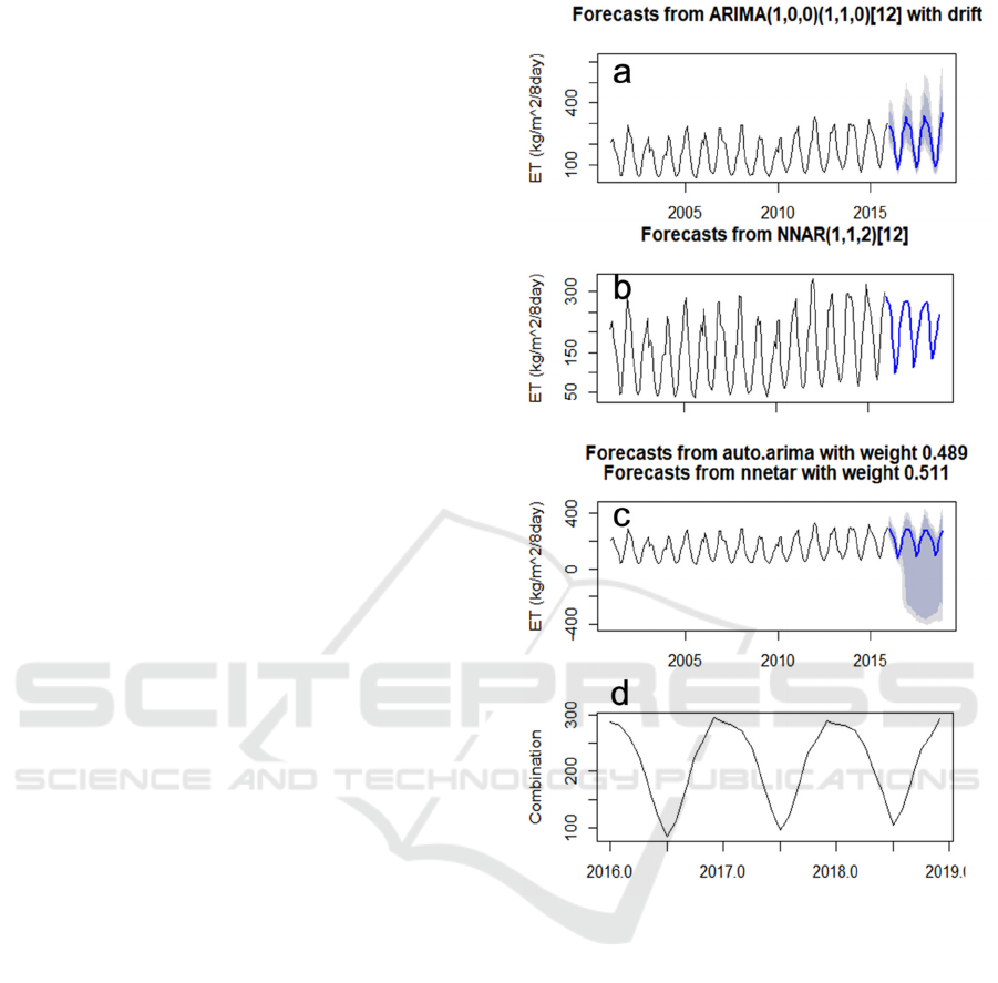
Figure 3(a-c) depicts the prediction results using
ARIMA, ANN and Hybrid models. After the training
of the models was done using 15 years time series
data from 2001 to 2015, the next step was to predict
ET using the remaining 3 year data from 2016 to
2018. Thus, the data set from 2016 to 2018 was used
as the testing part of the time series Prediction. This
was important in forecasting because the testing part
is forecasted and then forecasting results are
compared with the actual results. The black line
represents the training part of the time series data
(2001 to 2018) and the ET forecasted results (2016 to
2018) indicated by the blue line with the dark grey
and light-grey shadings, indicating the 80% and 95%
confidence levels of the forecasted time series. The
ARIMA model constructed for this data is the
ARIMA (1,0,0) and NNAR (1,1,2)(12) for ANNs.
The Zhang P. G., (2003) proposed this model
shown by figure 3(d) because of its the ability to
forecast both linear and nonlinear underlying
processes. The Kaiskammahoek irrigation scheme is
no exception to real world time series contains both
linear and nonlinear correlation structures. The black
line indicates the training data set for a 15-year period
(2001 to 2015); the blue line indicates the forecasted
ET
results, and the grey shading indicating the 95%
Figure 3: Forecasted ET for 3-year period from 2016 to
2018 using the ARIMA (a), ANN (b), Hybrid (ARIMA-
ANN) (c) and the ever-aged models (d). The black line in
Figure 3 (a-c) represents the data from 2001 to 2015 and the
blue line presents the 3 year forecast, with 95% confidence
levels grey lines (a &c) and figure 3(d) with a black line
representing 3 years averaged (ARIMA, ANN and Hybrid)
models.
confidence levels for the three year period (2016 to
2018).
Consecutively Figure 3(d) shows the prediction of
3 combined ARIMA, ANN and Hybrid models
averaged using the summation methods. The black
line shows combined prediction part from 3 models
used from 2016 to 2018. This was done to see if the 3
averaged models could improve the forecast as such
has been proven by other researchers. This study has
employed 3 different model systems and showed its
Evapotranspiration Prediction Using ARIMA, ANN and Hybrid Models for Optimum Water Use in Agriculture: A Case Study of
Keiskammahoek Irrigation Scheme, Eastern Cape, South Africa
281
performances in terms of the correlation coefficient
“R”. However, it is always important to also average
the forecast in order to improve the forecast accuracy
(Bates & Granger, 2017, Clemen, 1989).
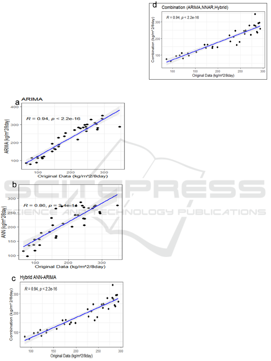
3.4 Correlation Statistics
To check the correlation of the prediction portion
person correlation (Lin, 1989), was employed with
ET predicted variables against the ET observed
variables. Figure 3 (a-d) depicts the scatter diagram
of the original ET and forecasted ET, represented by
the black dots falling on the 45 line through the origin.
Figure 4: Scatter plot between observed and forecasted ET
show diagram of the actual ET versus the forecasted annual
ET using ARI-MA (1,0,0)(1,1,0)[12] (a), NNAR(1,1,2)[12]
(b), Hybrid (ARIMA-ANN's) (c) and the averaged (d)
models (with validation period, 2016 to 2018).
The correlation of the forecasted for all the 4
forecasting models applied shows a strong correlation
coefficient with ARIMA (R = 0.94), ANN (R= 0.86),
Hybrid (R = 94) and the averaged models with (R =
0.94). Based on the R values for all the 3 models and
the averaged model, it is evidence that there is higher
linear relationship between the forecasted results and
the original time series data. Correlation Coefficient
suggest other 3 used forecasting modelling ARIMA
and Hybrid to be more correlated compared to lower
value of ANN (0.86).
3.5 Model Comparison
Table 1 below shows the three models employed in
this study to forecast ET at Keiskammahoek
Irrigation Scheme, namely ARIMA, ANNs and
Hybrid (ARIMA-ANN), and average of the three
models. The model forecast capabilities are compared
by using model performance statistics such as Root
Mean Square Error (RMSE), Mean Absolute Error
(MAE), Mean Absolute Percentage Error (MAPE),
and Correlation Coefficient (R). The results presented
in this table indicate that Hybrid model outperforms
other models with RMSE = 33.80, MAE = 27.02,
MAPE = 17.31 and R = 0.93. It is also noticeable that
the Mean Absolute Percentage Error-values for
ARIMA and Hybrid seem similar, considering
ARIMA (MAPE = 17.26) and Hybrid (MAPE =
17.31). Since the hybrid model is made up of a
combination of ARIMA and ANNs, it is possible that
this model will perform better than the other models
because it is expected to be capable of capturing both
linearity and non-linearity in the time series. In terms
of the correlation coefficient, ARIMA seems to
outperform the others models, with a correlation
coefficient of R = 0.94.
ISWEE 2022 - International Symposium on Water, Ecology and Environment
282

Table 1: Comparison of the ARIMA, ANN, Hybrid and
Combined Models: RMSE, MAE, MPE, and R.
Models RMSE MAE MAPE R
ARIMA 37.58 32.37 17.26 0.94
ANN 44.18 35.88 24.35 0.86
Hybrid 33.80 27.02 17.31 0.94
Combined 34.68 28.00 18.15 0.94
These results are interesting as they agree with
results found by (Zhang P. G., 2003), who archives
higher accuracy of time series prediction through use
of Hybrid (ARIMA-ANN) models.
The three utilized models were further averaged
to see if prediction accuracy could be reached. It has
been shown in previous studies that combination of
multiple forecasting methods leads to increase of the
forecasting accuracy (Clemen, 1989). Therefore, in
this study, the predictions obtained from the three
models used were combined by using the summation
method. The results of the COMBINED models
indicated in Table 1 show better results of ARIMA
and NNAR. These observations are encouraging as
they are consistent with results of studies on the
combination of several time series forecasting
methods. Similar what is obtained in this study,
Hyndman & Athanasopoulos, (2018), also pointed
out that combining forecasts often lead closer to, or
better than, the best component method.
4 CONCLUSIONS
The possibility to predict evapotranspiration (ET) is
essential as it can affirm perfect planning, design and
operation of any irrigation scheme. Thus, the main
aim of this study was to predict evapotranspiration
(ET) at Keiskammaheok, Irrigation Scheme located
in the province of Eastern Cape of South Africa using
3 time series forecasting models, namely (ARIMA),
(ANN), and the Hybrid (ARIMA-ANN) models. The
18 years (2001-2018) remotely sensed ET data was
extracted from a cloud-built software called Moderate
Resolution Imaging Spectroradiometer (MODIS)
Tera/ Aqua 16-day dataset. Using four model models
performance measures, namely, Root Mean Square
Error (RMSE), Mean Absolute Error (MAE), Mean
Absolute Percentage Error (MAPE), and the
Correlation Coefficient (R). It could be concluded
that the Hybrid (ARIMA-ANN) guarantees the
steadfast ET prediction for Keiskammahoek
irrigation Scheme. The model outperformed other
models with less values (RMSE =33.80, MAR =
27.02, MAPE = 17.31 and R = 0.94). This indicates
that the combination of ARIMA and ANN is a better
option because such hybrid models are able to capture
both linearity and non-linearity in the time series of
ET, which in turn produce better results. This work
will assist the Keiskammahoek irrigation scheme
management to plan effectively.
Future work may include further checking other
variables in order to assess whether these reported
drought in this region like Normalized Different
Vegetation Index (NDVI) to assess vegetation state,
Normalized Deference Water Index (NDWI) which is
the availability of water in plants and Normalized
Difference Different Index (NDDI) in order to check
the drought state in the study site.
ACKNOWLEDGEMENTS
This author like to thank Department of Higher
Education and Training (DHET) for funding the
project under its prestigious program named New
Generation of Academics Program (nGAP), and the
Manufacturing, Engineering and Related Services
SETA (merSETA) under the Walter Sisulu
University Faculty of Science, Engineering and
Technology (FSET).
The authors also would like to thank all personnel
involved in the development of the Google Earth
Engine system and climate engine. We also thank the
providers of the important public data set in the
Google Earth Engine, in particular NASA, USGS,
NOAA, EC/ESA, and MERRA-2 model developers.
REFERENCES
Adebiyi, A. A., Adewumi, A. O., & Ayo, C. K. (2015).
Comparison of Arima and Artificial Neural Networks
Models for Stock Price Prediction. Jornal of Applied
Mathamatics.
Adler, J., & Parmryd, I. (2010). Quantifying colocalization
by correlation: The Pearson correlation coefficient is
superior to the Mander's overlap coefficient. Journal of
Quantitative Cell Science.
Anapalli, S., Fisher, D. K., Reddy, K. N., Rajan, N., &
Pinnamaneni, S. R. (2019). Modeling
evapotranspiration for irrigation water management in
a humid climate. Agricultural Water management,
105731.
Evapotranspiration Prediction Using ARIMA, ANN and Hybrid Models for Optimum Water Use in Agriculture: A Case Study of
Keiskammahoek Irrigation Scheme, Eastern Cape, South Africa
283

Arnold, G. J., Srinivasan, R., Muttiah, S. R., & Williams, J.
R. (1998). Large area hydrologic modeling and
assessment part I: Model development. Journal of the
American water resources Association.
Averbeke, V. W., M'Marete, C. K., Belete, A., & Igodan,
C. O. (1998). An investigation into food plot production
at irrigation schemes in central eastern cape. Eastern
Cape: Water Research Commission Report.
Bachour, R. (2013). Evapotranspiration modeling and
forecasting for efficient management of irrigation
command areas. Doctoral dissertation, Utah State
University.
Bates, M. J., & Granger, J. W. (2017). The combination of
Forecast. Journal of the Operational reaserch Society.
Bencherif, H., Toihir, A. M., Mbatha , N., Sivakuma, V.,
Preez, D. J., beque, N., & Coetzee, G. (2020). Ozone
Variability and Trend Estimates from 20-year of
Ground-Based and Satellite Observations at Irene
Station, South Africa. MDPI atmosphere.
Botai, C. M., Botai, J., Adeola, A. M., Wit, J. P.,
Ncongwane, K. P., & Zwane, N. N. (2020). Drought
Risk Analysis in the Eastern Cape Province of South
Africa: The Copula Lens. Water.
Burns, P. (2002). Robustness of Ljung-Box Test and its
Rank. www.burns-stat.com.
Calzadilla, A., Zhu, T., Rehdanz, K., Richard, S. T., &
Ringler, C. (2014). Climate change and agriculture:
Impacts and adaptation options in South Africa.
Elsevier, 24-48.
Chai, T., & Draxler, R. R. (2014). Root mean square error
(RMSE) or mean absolute error (MAE)? – Arguments
against avoiding RMSE in the literature. European
Geosciences Union, 1247-1250.
Chersich, M. F., Wright, C. Y., Venter, F., Rees, H., Fiona,
S., & Erasmus, B. (2018). Impacts of Climate Change
on Health and Wellbeing in South Africa. International
Journal of Enviromental Research and Public Health.
Clemen, R. T. (1989). Combination Forecast: A review and
annotated bibliography. International Journal of
Forecasting, 559-583.
Contreras, J., Esponola, R., Nogales, F., & Conejo, A. J.
(2003). ARIMA Models to Predict Next-Day
Electricity Prices. IEEE Transactions of Power
Systems.
Dang, X., Peng, H., Wang, X., & Zhang, H. (2008). Theil-
Sen Estimators in a Multiple Linear Regression Model.
Olemiss Edu.
Darmawan, Y., & Sofan, P. (2012). Comparison of the
vegetation indices to detect the tropical rain forest
changes using breaks for additive seasonal and trend
(BFAST) model. International Journal of Remote
Sensing and Earth Sciences, 21-34.
Dinpashoh, Y., Jhajharia, D., Pard-Fakheri, A., Singh, P.
V., & Kahya, E. (2011). Trends in reference crop
evapotranspiration over Iran. Elsevier, 422-433.
Dutta, B., Smith, W. N., Grant, B. B., Pattey, E., &
Desjardins, C. L. (2016). Model development in DNDC
for the prediction of evapotranspiration and water use
in temperate field cropping systems. Elsevier, 9-25.
Elwasify, A. I. (2015). A Combined Model between
Artificial Neural Networks and ARIMA Models.
International Journal of Recent Research in Commerce
Economics and Management, 134-140.
Gautam, R., & Sinha, A. K. (2016). Time series analysis of
refrence crop evapotranspiration for Bokaro District,
Jharkhand, India. Journal of Water and Land
Development, 51-56.
Ghorbani, M. A., Kazempour, R., Chau, K.-W.,
Shamshirband, S., & Ghazvinei, P. T. (2018).
Forecasting pan evaporation with an integrated
artificial neural network quantum-behaved particle
swarm optimization model: a case study in Talesh,
Northern Iran. Journal, 1(12), 724-737.
Graw, V., Ghazaryan, G., Dali, K., Gomez, A. D., Abdel-
Hamid, A., Jordaan, A., . . . Dubovyk, O. (2017).
Drought Dynamics and Gegetation Productivity in
Different Land Management Systems of Eastern Cape,
South Africa- A Remoste Sensing Perspective. MDI
sustainability.
Grinsted, A., Moore, J., & Jevrejeva, S. (2004). Application
of the cross wavelet transform and wavelet coherence
to geophysical time series. Nonlinear Processes in
Geophysics, 561-566.
Gwate, O., Mantel, S. K., Pailmer, A. R., Gibson, L. A., &
Munch, Z. (2018). Measuring and modelling
evapotranspiration in a South African grassland:
Comparison of two improved Penman-Monteith
formulations. WATER SA.
Hyndman, R. J., & Athanasopoulos, G. (2018). Forecasting
Principles and Practice. Australia: Monash University.
Jha, K. G. (2007). Artificial Neural Networks and Its
Applications.
Jovanovic, N., Mu, Q., Bugan, D. R., & Zhao, M. (2015).
Dynamics of MODIS evapotranspiration in South
Africa. Water South Africa, 79-90.
Khair, U., Fahmil, H., Hakim, S. A., & Rahim, R. (2017).
Forecasting Error Calculation with Mean Absolute
Deviation and Mean Absolute percentage Error.
Journal of Physics.
Khanna, R., Plyus, & Bhalla, P. (2014). Study of Artificial
Neural Network. International Journal of Research in
Information technology, 271-276.
Khoshhal, J., & Mokarram, M. (2012). Model fpr
Prediction of Evapotranspiration Using MLP Neural
Network. International Journal of environmental
Science, 3.
Kishore, V., & Pushpalatha, M. (2017). Forecasting
Evapotranspiration for Irrigation Scheduling using
Neural Networks and ARIMA. International Journal of
Applied Engineering Research, 10841-10847.
Lewis, C. D. (1982). Industrial and business forecasting
methods: A practical guide to exponential smoothing
and curve fitting. Butterworth-Heinemann.
Lin, L. I.-K. (1989). A Consordance Correlation Coefficient
to Evaluate Reproducibility. International Biometric
Society is collaborating with JSTOR to digitize,
preserve and extend access to Biometrics, 255-268.
Loua, R. T., Bencherif, H., Mbatha, N., Begue, N.,
Hauchecome, A., Bamba, Z., & Sivakumar, V. (2019).
ISWEE 2022 - International Symposium on Water, Ecology and Environment
284

Study on Temporal Variations of Surface Temperature
and Rainfall at Conakry Airport, Guinea: 1960–2016.
MDPI.
Loua, R. T., Bencherif, H., Mbatha, N., Begue, N.,
Hauchecome, A., Bamba, Z., & Sivakumar, V. (2019).
Study on Temporal Variations of Surface temperiture
and Rainfall at Nonakry Airport, Guinea:1960-2016.
MDPI Climate.
Mahlalela, P. T., Blamey, R. C., Hart, N. C., & Reason, C.
J. (2020). Drought in the Eastern Cape region of South
Africa and trends in rainfall characteristics. Climate
Dynamics.
Maier, H. R., & Dandy, G. C. (2000). Neural networks for
the prediction and forecasting of water resources
variables: a review of modelling issues and
applications. Elsevier, 101-124.
Mallikarjuna, M., & Prabhakara, R. R. (2019). Evaluation
of forecasting methods from selected stock market
returns. Springer .
Mandleni, B., & Anim, F. (2011). Climate Change
Awareness and decision on Adaption Measures by
Livestock Famers. 85rd Annual Confrence of the
Agricultutre Economics Society. Florida: Warwick
University.
Mbatha, N., & Bencherif, H. (2020). Time Series Analysis
and Forecasting Using a Novel Hybrid LSTM Data-
Driven Model Based on Empirical Wavelet Transform
Applied to Total Column of Ozone at Buenos Aires,
Argentina (1966–2017). MD{I-Atmosphere.
Mbatha, N., & Xulu, S. (2018). Time Series Analysis of
MODIS-Derived NDVI for the Hluhluwe-Imfolozi
Park, South Africa: Impact of Recent Intense Drought.
MDPI-CLimate.
Mishra, A. K., & Singh, V. P. (2011). Drought Modeling.
Elsevier, 157-175.
Morimoto, T., Ouchi, Y., Shimizu, M., & Baloch, M. S.
(2007). Dynamic optimization of watering satsuma
mandarin using neaural networks and genetic
algorithms. Elsevier.
Mukaka, M. M. (2012). Statistics Corner: A guide to
appropriate use of Correlation coefficient in medical
research. Malawi Medical Journal, 69-71.
Myttenaere, A. D., Golden, B., Grand, B. L., & Rossi, F.
(2016). Mean Absolute Percentage Error for regression
models. Elsevier.
Ng, K. E., & Chan, C. J. (2012). Geophysical Applications
of Partial Wavelet Coherence and Multiple Wavelet
Coherence. Journal of Atmospheric and Ocean
Technolgy, 1845-1853.
Nkondo, M. N., Zyl, F. V., Keuris, H., & Shrener, B.
(2012). Proposed National Water Resoiurce Strategy
2(NWRS 2): Summary. Managing water for an
equitable and sustainable future. Department of Water
Affairs, Republic of South Africa.
Parasuraman, K., Elshorbagy, A., & Carey, S. K. (2007).
Modelling the dynamics of the evapotranspiration
process using genetic programming. hydrological
Sciences Journal, 563-578.
Patel, J. N., & Balve, P. N. (2016). Evapotranspiration
estimation with Fuzzy Logic. Proceedings of 40th The
IRES International Conference (pp. 20-23).
International Journal of Mechanical Civil Engineering.
Pohlert, T. (2017). Non-Parametric Trend Tests and
Change-Point Detection.
Rahimi, S., Sefidkouhi, M. A., Raeini-Sarjaz, M., &
Valipour, M. (2015). Estimation of actual
evapotranspiration by using MODIS images (a case
study: Tajan catchment). Archives of Agronomy and
Soil Science, 695-709.
Ramoelo, A., Majozi, N., Mathieu, R., Jovanivoc, N.,
Nickless, A., & Dzikiti, S. (2014). Validation of Global
Evapotranspiration Produc (MOD16) using Flux Tower
Data in the African Savanna, South Africa. Remote
sensing, 7406-7423.
Raymond, S. (1991). On the statistical analysis of series of
observations.
Reza, A. D., & Debnath, T. (2020). An approach to make
comparison of ARIMA and NNAR Models for
Forecasting Price of Commodities. Research Gate.
Sanral, Gibb, & Eoh. (2016). Improvement of national route
N2 Section 14&15 from green river (KM 60.0) to
Zwelitsha intersection (KM 6.00) & the new breidbach
interchange (KM 9.8). Eastern Cape: department of
Environmental Affairs Republic of South Africa.
Schultz, A., Wieland, R., & Lutze, G. (2000). Neural
networks in agroecological modelling — stylish
application or helpful tool? Elsevier, 73-97.
Soh, Y. W., Koo, C. H., Huang, Y. F., & Fung, K. F. (2018).
Application of artificial intelligence models for the
prediction of standardized precipitation
evapotranspiration index (SPEI) at langat River Basin,
Malaysia. Computer and Electronics in Agriculture,
164-173.
Todaro, M. P., & Smith, S. C. (2012). Economic
Development. New York: Library of Congress
Cataloging .
Todaro, M. P., & Smith, S. C. (2020). Economic
development. In M. P. Todaro, & S. C. Smith. Pearson:
library of congress ctaloging.
Torrence, C., & Compo, G. P. (1998). A practical guide to
wavelet analysis. Bulletin of American Meteorological
Society, 61-78.
Torrence, C., & Gompo, G. P. (1997). A Practical Guide to
Wavelet Analysis. Bulletin of the American
Meteorological Society.
Traore, S., Wang, Y.-M., & Kerh, I. (2008). Modeling
Reference Evapotranspiration by Generalized
Regression Neural Network in Semiarid Zone of
Africa. WSEAS Transactions on information science &
applications, 991-1000.
Valipour, M., Banihabib, M. E., & Behbahani, S. M.
(2013). Comparison of the ARMA, ARIMA and the
autoregressive artificial neural network models in
forecasting the monthly inflow of Dez dam reservoir.
Journal of Hydrology, 433-441.
Widowati, Putro, P. S., Koshio, S., & Oktaferdian, V.
(2016). Implementation of RIMA model to asses
Seasonal Variability Macrobenthic Assemblages.
Elsevier, 277-284.
Willmott, & Matsuura. (2005).
Evapotranspiration Prediction Using ARIMA, ANN and Hybrid Models for Optimum Water Use in Agriculture: A Case Study of
Keiskammahoek Irrigation Scheme, Eastern Cape, South Africa
285

Willmott, C. J., & Matsuura, K. (2005). Advantages of the
mean absolute error (MAE) over the root mean square
error (RMSE) in assessing average model performance.
climate research clim res, 79-82.
Yang, F., White, M. A., Michaelis, A. R., Ichii, K.,
Hashimoto, H., Votava, P., . . . Nemani, R. R. (2006).
Prediction of Continental-Scale Evapotranspiration by
Combining MODIS and AmeriFlux Data Through
Support Vector Machine. IEEE Transactions on
Geoscience and remote sensing.
Yue, S., & Wang, Y. C. (2004). The Mann-Kendall Test
Modified by Effective Sample Size to Detect Trend in
Serially Correlated Hydrological Series. Springer Link,
201-218.
Zhang, G., Patuwo, E. B., & Hu, Y. M. (1998). Forecasting
with artificial neural networks: The state of the art.
Elsevier, 35-62.
Zhang, L., Zhang, G. X., & Li, R. R. (2016). Water Quality
Analysis and Prediction Using Hybrid Time Series and
Neural Network Models. J.Agri.Sci. Tech, 975-983.
Zhang, P. G. (2003). Time series forecasting using a hybrid
ARIMA and Neural network model. Elsevier, 159-175.
Ziervogel, G., New, M., Archer, G. v., Midgley, G., Taylor,
A., Mamann, R., . . . Warburton, M. (2014). Climate
change impacts and adaption in South Africa. WIREs
Climate Change .
ISWEE 2022 - International Symposium on Water, Ecology and Environment
286
