
Energy Optimal Control of Collision Avoidance from Two Inertial
Objects
Pengfei Zhang, Hao Zhang, Feng Song and Yiqun Zhang
∗
Beijing Institute of Electronic System Engineering, Beijing, 100854, China
Keywords:
Optimal Control, Differential Games, Two vs One, Collision Avoidance.
Abstract:
Energy optimal control of collision avoidance is significant in aerospace and robotics. In this paper, we are to
investigate the energy optimal control problem of avoiding collision from two inertial objects, in a differential
game manner. In particular, we develop the optimal control structure by applying the already published payoff
augmentation method, and the result shows that the control of the evader is zero in some time periods. For
verification, a simulation case is constructed and the results are consistent with the theoretical analysis.
1 INTRODUCTION
The study of energy optimal control is significant
in collision avoidance problems. The problem can
be solved by regarding it as a pursuit evasion game
(Bas¸ar and Zaccour, 2018; Friedman, 2013), in which
the obstructive objects are assumed to be intelligent.
Pursuit evasion games are widely used in aerospace,
collision avoidance, robotics (Isaacs and Philip, 1966;
Exarchos et al., 2015; Exarchos et al., 2016; Kumkov
et al., 2014). In a pursuit evasion game, the pursuer
tries to approach the evader, while the evader avoids
collision with the pursuer. In many cases, there might
be more than one obstructive objects, and the evader
has to design its optimal control taking all the obstruc-
tive objects into consideration. The problem becomes
the well known two pursuers one evader game when
two obstructive objects exist, which is to be investi-
gated in this paper.
Two pursuers and one evader game is more diffi-
cult than one pursuer and one evader game (Ganebny
et al., 2012; Garcia et al., 2017; Exarchos et al.,
2016), for the payoff function has a more complex
form. When considering the energy optimal control
problem, the energy term should be included in the
payoff function. Extensive studies have researched
the two pursuers and one evader differential games,
among which the linear dynamic model and simple
motion model of the players are mostly considered
(Le M
´
enec, 2011; Garcia et al., 2017; Makkapati
et al., 2018; Ganebny et al., 2012; Hagedorn and
Breakwell, 1976; Ho et al., 1965; Kumkov et al.,
2014; Pachter et al., 2020; Pachter et al., 2019; Sun
et al., 2017). For the linear dynamic model game, the
zero effort miss approach is widely adopted, which
brings remarkable convenience. For the simple mo-
tion games (Garcia et al., 2017; Makkapati et al.,
2018; Pachter et al., 2020; Pachter et al., 2019), it has
shown the most of the optimal controls are moving
straight. When facing the inertial model two pursuers
one evader games, Zhang et.al has analysed the time
optimal problem by proposing a payoff augmentation
method and an open loop Stackelberg approach. This
paper will analyse the energy optimal problem by
the method proposed by the reference (Zhang et al.,
2022).
In this paper, we study the energy optimal con-
trol of avoiding collision from two inertial objects, in
a differential game manner. It is assumed that our
flying vehicle (the evader) is hit by the obstructive
objects when their distance is less than l. We adopt
the payoff augmentation method introduced by refer-
ence (Zhang et al., 2022) to obtain the optimal control
form. As a result, it will be shown that the energy op-
timal control problem has a different result with the
time optimal problem. The major difference is that
the evader adopts zero control in some time periods,
which is consistent with intuition.
Zhang, P., Zhang, H., Song, F. and Zhang, Y.
Energy Optimal Control of Collision Avoidance from Two Inertial Objects.
DOI: 10.5220/0012016200003612
In Proceedings of the 3rd International Symposium on Automation, Information and Computing (ISAIC 2022), pages 681-685
ISBN: 978-989-758-622-4; ISSN: 2975-9463
Copyright
c
2023 by SCITEPRESS – Science and Technology Publications, Lda. Under CC license (CC BY-NC-ND 4.0)
681

2 PROBLEM STATEMENT
2.1 State Equation
Three players move on a planar. One is the evader, the
rest two are the pursuers P1 and P2. The evader sur-
vives should the distance of the evader and the closest
pursuer is bigger or equal than l. Th game operates
in the time interval [0,T ]. The three players have in-
ertial dynamic models controlled by acceleration vec-
tors, written as
˙x
p1
= v
p1
x
˙y
p1
= v
p1
y
˙v
p1
x
= a
1
cosu
1
˙v
p1
y
= a
1
sinu
1
,
˙x
p2
= v
p2
x
˙y
p2
= v
p2
y
˙v
p2
x
= a
2
cosu
2
˙v
p2
y
= a
2
sinu
2
,
˙x
e
= v
e
x
˙y
e
= v
e
y
˙v
e
x
= a
3
cosu
3
˙v
e
y
= a
3
sinu
3
(1)
where the supscripts pi and e are used for the i-th pur-
suer and the evader respectively. x, y are the positions,
v
x
, v
y
are the velocities. a
1
∈ [0,a
1m
], a
2
∈ [0,a
2m
]
and a
3
∈ [0,a
3m
] are the magnitudes of the accelera-
tion vectors. u
1
, u
2
and u
3
represent the headings of
the acceleration vectors of P1, P2 and E.
To obtain a reduced system, new variables are in-
troduced
x
1
= x
p1
−x
e
y
1
= y
p1
−y
e
v
1x
= v
p1
x
−v
e
x
v
1y
= v
p1
y
−v
e
y
x
2
= x
p2
−x
e
y
2
= y
p2
−y
e
v
2x
= v
p2
x
−v
e
x
v
2y
= v
p2
y
−v
e
y
(2)
where x
1
,y
1
,v
1x
,v
1y
,x
2
,y
2
,v
2x
,v
2y
represent the rela-
tive positions and velocities.
Based on (2), (1) is rewritten as
˙x
1
= v
1x
˙y
1
= v
1y
˙v
1x
= a
1
cosu
1
−a
3
cosu
3
˙v
1y
= a
1
sinu
1
−a
3
sinu
3
˙x
2
= v
2x
˙y
2
= v
2y
˙v
2x
= a
2
cosu
2
−a
3
cosu
3
˙v
2y
= a
2
sinu
2
−a
3
sinu
3
(3)
The payoff function is the evader’s cost energy,
under the state constraint that the distance of the
evader and the pursuers are ≥l in whole game period.
In particular, the payoff function is written as
J =
T
Z
0
a
3
dt (4)
The evader wishes to minimize Eq. (4), while the
pursuer has the opposite purpose. The state constraint
is written as:
min
t∈[0,T ]
q
x
2
1
(t) + y
2
1
(t) ≥ l
min
t∈[0,T ]
q
x
2
2
(t) + y
2
2
(t) ≥ l
(5)
where the evader has to make (5) hold while the pur-
suers wishes the opposite.
3 ANALYSIS OF OPTIMAL
CONTROL
With the aid of the method proposed in reference
(Zhang et al., 2022), the new payoff function is de-
signed as
J =
T
Z
0
[a
3
+
1
k
1
e
k
2
1
(l
2
−x
2
1
−y
2
1
)
+
1
k
2
e
k
2
2
(l
2
−x
2
2
−y
2
2
)
]dt (6)
where k
1
approaches +∞, k
2
approaches +∞.
As what we have anticipated, the game is trans-
formed to a new game of degree with payoff function
(6).
Based on the state equation (3), the Hamiltonian
function is written as
H = a
3
+
1
k
1
e
k
2
1
(l
2
−x
2
1
−y
2
1
)
+
1
k
2
e
k
2
2
(l
2
−x
2
2
−y
2
2
)
+λ
1
v
1x
+ λ
2
v
1y
+ λ
3
(a
1
cosu
1
−a
3
cosu
3
)
+λ
4
(a
1
sinu
1
−a
3
sinu
3
)
+λ
5
v
2x
+ λ
6
v
2y
+ λ
7
(a
2
cosu
2
−a
3
cosu
3
)
+λ
8
(a
2
sinu
2
−a
3
sinu
3
)
(7)
where λ
i
(i = 1,2,...,8) are co-states.
Based on (7), the co-state equation is derived as
˙
λ
1
= 2k
1
x
1
e
k
2
1
(l
2
−x
2
1
−y
2
1
)
˙
λ
2
= 2k
1
y
1
e
k
2
1
(l
2
−x
2
1
−y
2
1
)
˙
λ
3
= −λ
1
˙
λ
4
= −λ
2
˙
λ
5
= 2k
2
x
2
e
k
2
2
(l
2
−x
2
2
−y
2
2
)
˙
λ
6
= 2k
2
y
2
e
k
2
2
(l
2
−x
2
2
−y
2
2
)
˙
λ
7
= −λ
5
˙
λ
8
= −λ
6
(8)
Since the pursuers maximizes H and the evader
minimizes H in (7), the control equations are written
as
a
1
= a
1m
,cosu
1
=
λ
3
√
λ
3
2
+λ
4
2
,sinu
1
=
λ
4
√
λ
3
2
+λ
4
2
a
2
= a
2m
,cosu
2
=
λ
7
√
λ
7
2
+λ
8
2
,sinu
2
=
λ
8
√
λ
7
2
+λ
8
2
a
3
=
(
a
3m
,when 1−
q
(λ
3
+ λ
7
)
2
+ (λ
4
+ λ
8
)
2
< 0
0,else
cosu
3
=
λ
3
+λ
7
√
(λ
3
+λ
7
)
2
+(λ
4
+λ
8
)
2
,sinu
3
=
λ
4
+λ
8
√
(λ
3
+λ
7
)
2
+(λ
4
+λ
8
)
2
(9)
ISAIC 2022 - International Symposium on Automation, Information and Computing
682

Suppose that at time t
2
and time t
1
, P2 and P1 at-
tain their minimum distance l with E, that is x
2
1
(t
1
) +
y
2
1
(t
1
) = l
2
and x
2
2
(t
2
) + y
2
2
(t
2
) = l
2
. Without loss of
generality, we assume that t
1
≤t
2
.
a) Case t
1
< t
2
Since there are no terminal constraints on the
state variables, we conclude that λ
i
(T ) = 0(i =
1,2,..., 8). Based on (8), in the time interval
(t
2
,T ], the derivatives of the co-states approach
zero as k
1
and k
2
approach +∞. Therefore, the
co-states in the time interval (t
2
,T ] are written as:
λ
i
(τ) = 0, i = 1,2, ...,8
(10)
where τ ∈ (t
2
,T ].
At time t
2
, it can be seen from (8) that
˙
λ
5
and
˙
λ
6
are not zero when k
2
approaches +∞. Thereby, in
the time interval (t
1
,t
2
], the co-states are derived
as:
λ
i
(τ) = 0, i = 1,2, 3,4
λ
5
(τ) = −2k
2
x
2
(t
2
)dt
λ
6
(τ) = −2k
2
y
2
(t
2
)dt
λ
7
(τ) = −2k
2
x
2
(t
2
)dt(t
2
−τ)
λ
8
(τ) = −2k
2
y
2
(t
2
)dt(t
2
−τ)
(11)
where τ ∈ (t
1
,t
2
].
At time t
1
, it can be seen from (8) that
˙
λ
1
and
˙
λ
2
are not zero when k
1
approaches +∞. Thereby, in
the time interval [0 t
1
], the co-states are derived
as:
λ
1
(τ) = −2k
1
x
1
(t
1
)dt
λ
2
(τ) = −2k
1
y
1
(t
1
)dt
λ
3
(τ) = −2k
1
x
1
(t
1
)dt(t
1
−τ)
λ
4
(τ) = −2k
1
y
1
(t
1
)dt(t
1
−τ)
λ
5
(τ) = −2k
2
x
2
(t
2
)dt
λ
6
(τ) = −2k
2
y
2
(t
2
)dt
λ
7
(τ) = −2k
2
x
2
(t
2
)dt(t
2
−τ)
λ
8
(τ) = −2k
2
y
2
(t
2
)dt(t
2
−τ)
(12)
where τ ∈ [0,t
1
].
Since P1 and P2 respectively attain minimum dis-
tance with E at time t
1
and t
2
, the derivatives of
x
2
1
(t
1
) + y
2
1
(t
1
) and x
2
2
(t
2
) + y
2
2
(t
2
) are zero, yield-
ing
x
1
(t
1
)v
1x
(t
1
) + y
1
(t
1
)v
1y
(t
1
) = 0
x
2
(t
2
)v
2x
(t
2
) + y
2
(t
2
)v
2y
(t
2
) = 0
(13)
b) Case t
1
= t
2
In this case, the co-states in the time interval [0,
t
1
] are derived as:
λ
1
(τ) = −2k
1
x
1
(t
1
)dt
λ
2
(τ) = −2k
1
y
1
(t
1
)dt
λ
3
(τ) = −2k
1
x
1
(t
1
)dt(t
1
−τ)
λ
4
(τ) = −2k
1
y
1
(t
1
)dt(t
1
−τ)
λ
5
(τ) = −2k
2
x
2
(t
1
)dt
λ
6
(τ) = −2k
2
y
2
(t
1
)dt
λ
7
(τ) = −2k
2
x
2
(t
1
)dt(t
1
−τ)
λ
8
(τ) = −2k
2
y
2
(t
1
)dt(t
1
−τ)
(14)
(11), (12) and (14) provide the expressions of the
co-states. Based on the control equation in (9), the
equilibrium strategies are obtained as below.
Based on (9), (11), (12) and (14), we infer that
the pursuers adopt constant control. The magnitude
and heading of the pursuer’s acceleration are invari-
ant. Specifically, the best strategies of the pursuers
are written as
a
1
= a
1m
u
1
= ϑ
1
a
2
= a
2m
u
2
= ϑ
2
(15)
where ϑ
1
= arctan2 [−y
1
(t
1
),−x
1
(t
1
)],ϑ
2
=
arctan2 [−y
2
(t
2
),−x
2
(t
2
)].
Based on (9), the control of the evader a
3
and u
3
depend on the values of λ
3
+ λ
7
and λ
4
+ λ
8
. The
strategy of the evader is given in two cases as below.
a) Case t
1
< t
2
In the time interval (t
1
, t
2
], based on (11) and Eq.
(9), the control a
3
and u
3
are written as:
a
3
=
a
3m
,when 1 −|2k
2
dt(t
2
−τ)l| < 0
0,else
u
3
= ϑ
2
(16)
where τ ∈ (t
1
,t
2
].
In the time interval [0, t
1
], based on (12) and (9),
the control a
3
and u
3
are derived as:
a
3
=
a
3m
,when 1 −2ldt
v
u
u
u
u
t
k
2
1
(t
1
−τ)
2
+k
2
2
(t
2
−τ)
2
+2k
1
k
2
(t
1
−τ)
(t
2
−τ) cos(ϑ
1
−ϑ
2
)
< 0
0,else
u
3
= arctan2 [n,m]
where :
m = 2k
1
ldt(t
1
−τ) cos ϑ
1
+ 2k
2
ldt(t
2
−τ) cos ϑ
2
n = 2k
1
ldt(t
1
−τ) sin ϑ
1
+ 2k
2
ldt(t
2
−τ) sin ϑ
2
(17)
where τ ∈ [0,t
1
].
b) Case t
1
= t
2
In the time interval [0, t
1
], based on (14) and (9),
the controls are derived as:
a
3
=
a
3m
,when 1 −2ldt
v
u
u
u
t
(t
1
−τ)
2
k
2
1
+ k
2
2
+2k
1
k
2
cos(ϑ
1
−ϑ
2
)
< 0
0,else
u
3
= arctan 2 [n,m]
where :
m = (2k
1
ldt cosϑ
1
+ 2k
2
ldt cosϑ
2
)(t
1
−τ)
n = (2k
1
ldt sinϑ
1
+ 2k
2
ldt sinϑ
2
)(t
1
−τ)
(18)
where τ ∈ [0,t
1
]. It can be seen that u
3
is constant
in this case.
In a quick summary, (15), (16), (17) and (18)
present the equilibrium strategy structure of the dif-
ferential game. To solve the game when given an ini-
tial state, a two point boundary problem formulated
Energy Optimal Control of Collision Avoidance from Two Inertial Objects
683
by the state equation (3), the co-state equation (8) and
the control equation (9) needs to be calculated.
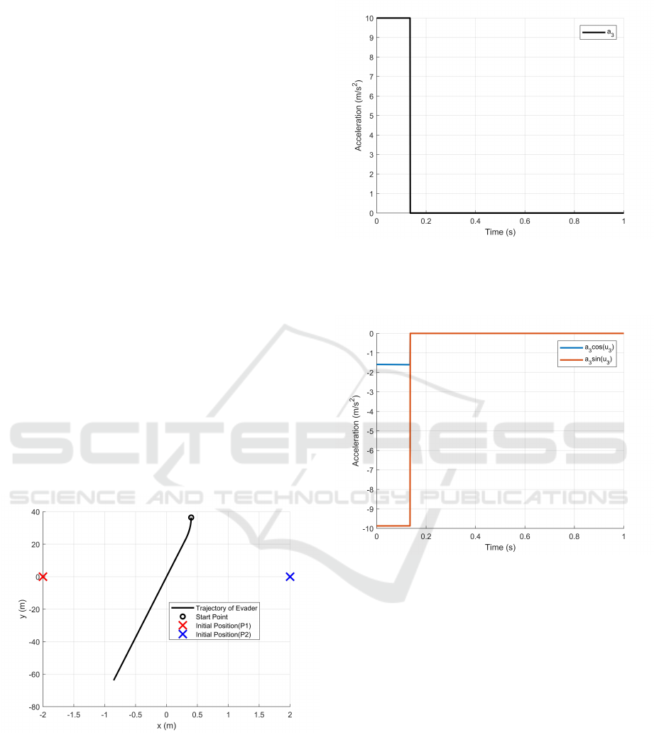
4 SIMULATION CASE
In this section, we present a simulation case. The end
time T = 1(s), the collision distance l = 1(m), the
bounds of the accelerations a
1m
= 15(m/s
2
),a
2m
=
15(m/s
2
),a
3m
= 10(m/s
2
). The initial position of the
evader is (0.4 m, 36.5 m), the initial velocity of the
evader is (0 m/s, -100 m/s). The initial positions of
the pursuers are (-2 m, 0 m) and (2 m, 0 m), the initial
velocities of the pursuers are (0 m/s, 0 m/s). By solv-
ing the two point boundary problem, the parameters
are calculated:
ϑ
1
= −0.086
ϑ
2
= −3.006
k
1
dt = 0.1472
k
2
dt = 2.3073
t
1
= 0.365
t
2
= 0.366
(19)
Based on the control equation of the evader, it is
derived that a
3
= 0 after time 0.135 s. The trajectory
of the evader is shown in Fig. 1. The evader turns
at first and then goes straight. The trajectory almost
passes by the point (0, 0), which locates at the middle
of the initial positions of the two pursuers.
Figure 1: The trajectory of the evader.
The magnitude of the acceleration of the evader a
3
with respect to time is shown in Fig. 2. The evader
adopts a
3
= 10 at first. After time 0.135 s, the evader
adopts a
3
= 0, indicating that the evader travels on a
straight line. Thus, the control effort (the integral of
a
3
in (4)) equals to 1.35.
The variation of the acceleration vector of the
evader – (a
3
cosu
3
,a
3
sinu
3
) – with respect to time is
Figure 2: The magnitude of the acceleration of the evader.
shown in Fig. 3. It is almost a constant vector before
time 0.135 s.
Figure 3: The variation of the acceleration vector of the
evader with respect to time.
The distance of the evader and the two pursuers
are shown in Fig. 4. The two distances attain their
minimum at the time 0.365 s and 0.366 s, which is
consistent with the values of t
1
and t
2
in (19). The
minimum of the distance is almost 1 m.
5 CONCLUSIONS
This paper investigated how to avoid collision with
two inertial obstructive objects by minimum energy
cost. Thanks to the payoff augmentation method
proposed by previous literature, the optimal control
structure is obtained, as well as a two point bound-
ary value problem established. A simulation was pre-
sented, and the result agree with the theoretical anal-
ysis.
ISAIC 2022 - International Symposium on Automation, Information and Computing
684
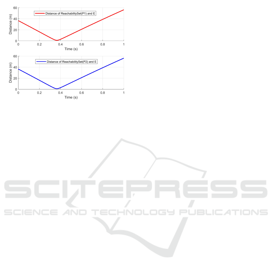
Figure 4: The distance of the evader and the reachability
sets of the two pursuers.
In the future, we may focus on studying the colli-
sion avoidance issue with more sophisticated dynamic
models.
ACKNOWLEDGMENTS
This work is supported, in part, by the NSFC
62088101 Autonomous Intelligent Unmanned Sys-
tems, and by the Zhejiang Provincial Natural Science
Foundation of China (Grant No. LR20F030003).
REFERENCES
Bas¸ar, T. and Zaccour, G. (2018). Handbook of dynamic
game theory. Springer.
Exarchos, I., Tsiotras, P., and Pachter, M. (2015). On the
suicidal pedestrian differential game. Dynamic Games
and Applications, 5(3):297–317.
Exarchos, I., Tsiotras, P., and Pachter, M. (2016). Uav col-
lision avoidance based on the solution of the suicidal
pedestrian differential game. In AIAA Guidance, Nav-
igation, and Control Conference, page 2100.
Friedman, A. (2013). Differential games. Courier Corpora-
tion.
Ganebny, S. A., Kumkov, S. S., M
´
enec, S. L., and Patsko,
V. S. (2012). Model problem in a line with two pur-
suers and one evader. Dynamic Games and Applica-
tions.
Garcia, E., Fuchs, Z. E., Milutinovic, D., Casbeer, D. W.,
and Pachter, M. (2017). A geometric approach for the
cooperative two-pursuer one-evader differential game.
Ifac Papersonline, 50(1):15209–15214.
Hagedorn, P. and Breakwell, J. V. (1976). A differential
game with two pursuers and one evader. Journal of
Optimization Theory & Applications, 18(1):15–29.
Ho, Y., Bryson, A., and Baron, S. (1965). Differential
games and optimal pursuit-evasion strategies. IEEE
Transactions on Automatic Control, 10(4):385–389.
Isaacs and Philip, R. (1966). Differential games : a math-
ematical theory with applications to warfare and pur-
suit, control and optimization. Wiley.
Kumkov, S. S., M
´
enec, S. L., and Patsko, V. S. (2014). Solv-
ability sets in pursuit problem with two pursuers and
one evader. Ifac Proceedings Volumes, 47(3):1543–
1549.
Le M
´
enec, S. (2011). Linear differential game with two pur-
suers and one evader. In Advances in dynamic games,
pages 209–226. Springer.
Makkapati, V. R., Sun, W., and Tsiotras, P. (2018). Pursuit-
evasion problems involving two pursuers and one
evader. In 2018 AIAA Guidance, Navigation, and
Control Conference, page 2107.
Pachter, M., Moll, A. V., Garcia, E., Casbeer, D., and Mi-
lutinovi, D. (2020). Cooperative pursuit by multiple
pursuers of a single evader. Journal of Aerospace In-
formation Systems, (2):1–19.
Pachter, M., Von Moll, A., Garcia, E., Casbeer, D. W., and
Milutinovi
´
c, D. (2019). Two-on-one pursuit. Journal
of Guidance Control & Dynamics, pages 1–7.
Sun, W., Tsiotras, P., Lolla, T., Subramani, D. N., and Ler-
musiaux, P. F. (2017). Multiple-pursuer/one-evader
pursuit–evasion game in dynamic flowfields. Journal
of guidance, control, and dynamics, 40(7):1627–1637.
Zhang, Y., Zhang, P., Wang, X., Song, F., and Li, C. (2022).
A payoff augmentation approach to two pursuers and
one evader inertial model differential game. IEEE
Transactions on Aerospace and Electronic Systems.
Energy Optimal Control of Collision Avoidance from Two Inertial Objects
685
