
Development of Input-Output Hidden Markov Model for Estimating
Diabetes Progression
Tianbei Zhang
University of California, Irvine, CA 92697, U.S.A.
Keywords: HMM, Diabetes.
Abstract: Incessant unhealthy routines are believed to induce chronic diseases. However, current modelling can barely
estimate diabetes progression by analyzing daily behaviours. In this study, an input-output hidden markov
model (iohmm) was constructed to forecast the progression of diabetes mellitus based on ordinary routines and
to reveal the association among illness indicators (e.g., blood glucose levels), living habits and medical
interventions. The analysis of diabetes datasets from the ucirvine machine learning repository revealed that the
high amount of food intake, insulin overdose and unideal health status could increase the risk of severe
exacerbation in diabetes patients. It was also found that the variation of blood glucose increased as the patients’
health conditions worsened. Besides, among all the factors tested in this study, the patients' initial health
conditions contributed the most to blood sugar fluctuation, while minor contributions from meal and insulin
were still effective enough to be regarded as significant factors. The proposed iohmm model enables the
inference of patient’s health conditions by analyzing their living habits. Most importantly, this study
successfully developed a novel iohmm model to estimate diabetes progression, which can be generalized and
applied to other chronic diseases.
1 INTRODUCTION
As a serious public health concern, type 2 diabetes
mellitus has led to over one million deaths in 2017
worldwide, making it the ninth leading cause of death
(Khan et al. 2020). A growing body of
epidemiological evidence indicates that there is an
urgent need to develop an effective method for
treating and preventing this disease. A study
conducted by Moien Khan and his colleagues
suggests that the prevalence of type 2 diabetes can
increase from 6059 cases per 100,000 in 2017 to 7862
cases per 100,000 by 2040 (Khan et al. 2020). Their
study also points to a shift in patient age, which
results in higher incidence rates in younger age
groups. Such increasing trends emphasize the
necessity of monitoring disease progression to
prevent this chronic disease (Divers et al. 2020). One
possibly effective method to treat and prevent type 2
diabetes is by estimating the disease progression,
which enables potential type 2 diabetes patients to
become aware of their blood glucose levels and take
corresponding precautions against this disease. To
make this form of surveillance and prevention, a
statistical model can be developed based on the daily
food consumption and blood samples collected from
screening tests. The existing models, such as Hidden
Markov model (HMM) and linear regression model,
can be used to predict early diabetes progression, but
their outcomes may not accurately reflect
intervariable correlations under some circumstances.
Since the HMM is not able to assess the effect of
inputs, it fails to represent the correct causal relation
between inputs and outputs. Thus, in this study, an
input and output hidden Markov model (IOHMM)
model was constructed, and an Expectation-
Maximization (EM) algorithm was used to remedy
the problems in current models.
Different from HMM and linear regression
model, IOHMM is a dynamic system designed for
forward and backward propagation in time to target a
discrete state space (Grover et al. 2013). In this study,
the IOHMM model provides a scalable framework to
represent the complex patterns of diabetes
progression. As a hidden variable in our model, the
patient’s health condition is estimated through
observable information. More importantly, the
proposed model can track and estimate illness
conditions temporally for each individual patient.
Apart from those advantages, an EM algorithm that
Zhang, T.
Development of Input-Output Hidden Markov Model for Estimating Diabetes Progression.
DOI: 10.5220/0012018600003633
In Proceedings of the 4th International Conference on Biotechnology and Biomedicine (ICBB 2022), pages 215-222
ISBN: 978-989-758-637-8
Copyright
c
2023 by SCITEPRESS – Science and Technology Publications, Lda. Under CC license (CC BY-NC-ND 4.0)
215

has great scalability can be applied to optimize our
model. This algorithm helps in finding optimal
parameters through iterative computation (Dempster
and Rubin 1977). Our study demonstrates the
potential application of IOHMM for estimating
diabetes progression. Depending upon the personal
results obtained from our model, a specific targeted
therapy can be provided to target patient’s needs.
2 METHODS
2.1 Data Description
The dataset used in this study is a diabetic patient
record published by the University of California,
Irvine’s Machine Learning Repository. The original
dataset was collected in 1994 by a PhD student,
Michael Kahn, from Washington University. This
dataset is composed of quantitative records (e.g.,
insulin doses, insulin types, and blood glucose levels
and categorical information (e.g., the size of meal
ingestion, regular physical activity and other living
routines) lasting at least three months for each of the
70 diabetes patients.
Since not all the variables were regularly
recorded, only three well-recorded variables were
acquired from this dataset: blood glucose level (g),
meal intake size (m), and units of insulin injected (i).
Among them, insulin injection (i) and food intake (m)
are sets of numerical data that have units of
treatments received by each patient. Blood glucose
level is a quantitative variable as well, which reflects
the patients’ health conditions.
2.2 Model Development
In this study, the association among variables was
revealed and the reliable projections were realized by
constructing the input and output HMM. Not only the
observed variables (e.g., food intake) were included
in this model, but also the hidden states such as
patients' health conditions (h) over time. From degree
one to eight, the variable h quantifies patients’ health
conditions from the healthiest to the worst. This latent
variable is structured to be influenced by its previous
day health conditions, food intake, and insulin
injection dose on the same day (Fig. 1). Such an
association could generate outcomes to indicate the
daily changes in health conditions. As shown in the
heatmap (Fig. 2), the probabilities of patients having
various physical conditions were expected to be
different. Additional treatments were also included to
evaluate the impact of other factors on transition
probabilities in actual model running.
As opposed to hidden factor h, blood glucose
levels are measurable and can be used to reflect the
changes in regular physical activity and patient’s
daily habits (Fig. 1). By giving treatments, an
emission relationship was expected to be observed.
For example, when increasing the amount of food
ingestion, the blood sugar levels could be higher with
a broader range compared to the control group (Fig.
3). For patients receiving excessive amount of
insulin, they may develop a higher chance of having
lower and unstable blood glucose levels (Fig. 3).
Apart from the assumptions of intervariable
association, model parameter development is another
indispensable step.
There are three parameters that contributed to our
model λ (π, φ, ψ): the prior, π, transition probability,
φ, and emission probability, ψ. The prior parameter
(π) which represents the health condition of our
samples on day 0 is an estimated value ((Equation
(1)). The transition parameter φ, as denoted by
Equation (2), is used to estimate the next health
condition state given previous disease progression,
current insulin injection doses, and current meal size.
Compared with the transition parameter, the emission
parameter, which estimates the probability of having
a certain blood glucose level on specific health
conditions, is constituted by pre-prandial and
postprandial emission parameters (Equations (3) and
(4)). The pre-prandial emission calculates the
probability of having certain pre-prandial glucose
levels based on the patient’s health conditions
(Equation (3)). In Equation (4), the postprandial
glucose level is estimated based on the performance
of patient’s health conditions, pre-prandial blood
glucose, insulin dose and food intake. Coefficients a,
b, c, d and μ were introduced to adjust and quantify
the impact of additional variables. In this study, we
assume that both transition and emission parameters
follow Gaussian distribution. However, further
studies are needed when the parameters are limited
for other specific distribution patterns.
𝜋
𝑘
= 𝑃
ℎ
= 𝑘
(1)
𝜑ℎ
ℎ
, 𝑖
,
, 𝑚
,
=
1
2𝜋𝜎
exp−
ℎ
+ 𝑑
,
⋅ 𝑖
,
− 𝑒
,
⋅ 𝑚
,
− 𝜇
2𝜎
(2)
𝜑𝑔
, ,
ℎ
=
1
2𝜋𝜎
,
,
exp−
𝑔
, ,
− 𝜇
,
2𝜎
,
,
(3)
ICBB 2022 - International Conference on Biotechnology and Biomedicine
216
𝜓𝑔
,,
ℎ
,𝑔
,,
,𝑖
,
,𝑚
,
=
1
2𝜋𝜎
,,
exp−
𝑔
,,
+𝑎
,
⋅𝑖
,
−𝑏
,
⋅𝑚
,
−𝑐
,
⋅𝑔
,,
−𝜇
,
2𝜎
,
,
(4)
The likelihood of our model, which indicates the
probability of having certain health conditions by
fitting the given model parameters (e.g., insulin
injection and food intake) at day t, is equal to the
product of the prior, sum of the transition
probabilities and sum of the emission probabilities at
different days (Equation (5)).
𝑝
ℎ,𝑔
|
𝑖,𝑚,𝜃
=𝜋
ℎ
∏
𝜑ℎ
ℎ
,𝑖
,
,𝑚
,
∏
𝜓𝑔
,,
ℎ
𝜓𝑔
,,
ℎ
,𝑔
,,
,𝑖
,
,𝑚
,
(5)
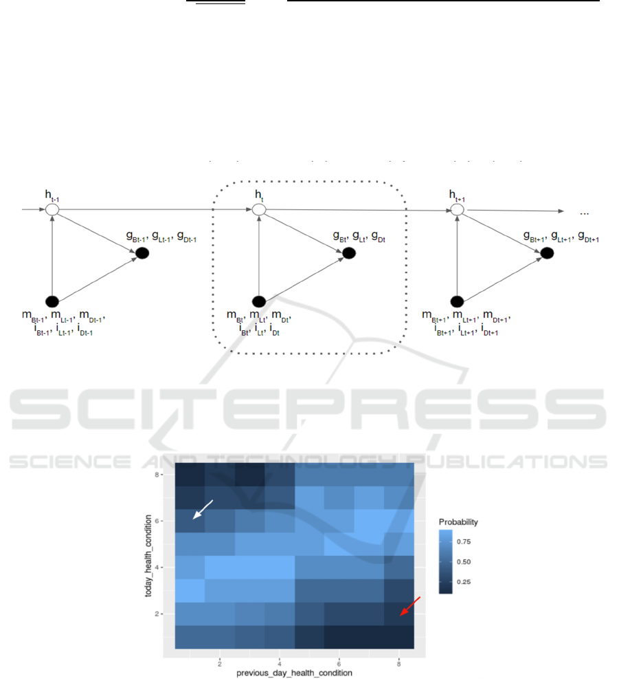
Figure 1: IOHMM demonstrating the relationship between observational measurements (denoted by black circles) and hidden
information (denoted by white circles). The arrows represent the associations among variables by pointing at outcome
variables from causal variables. This model establishes the relationships among health conditions (h), blood glucose levels
(g), meal intake sizes (m), and insulin injection doses (i). For meal intake size and insulin injection dose, daily (t)
measurements were conducted after breakfast (B), lunch (L), and dinner (D).
Figure 2: The expected transition probability distribution. The color shade in this heat map is used to visualize the probabilities
of having certain health conditions in the next stage. As the white arrow points at, for patients with lower previous day heath
conditions (healthier), they are anticipated to have higher chances to keep healthy conditions on the subsequent days. In
contrast, as indicated by the red arrow, patients with unideal previous day conditions are expected to have worse physical
circumstances over time.
Development of Input-Output Hidden Markov Model for Estimating Diabetes Progression
217

Figure 3: The expected emission outcomes. The probabilities of having different blood glucose levels when receiving various
treatments are expected to be observed.
2.3 Model Optimization
In order to optimize model parameters, the EM
algorithm was adopted to alternatively estimate the
posterior probability of latent states and update the
parameters in our model. Estimation was made by
EM algorithm based on the incomplete datasets
through iterative computation to maximize the
likelihood in two steps: expectation and
maximization steps. In our model, the formula of the
EM algorithm can be denoted by Equation (6).
(Dempster et al.).
𝜃
=
𝑃
ℎ
|
𝑔,𝑖,𝑚,𝜃
log𝑃
𝑔,𝑖,𝑚,ℎ
|
𝜃
𝑑ℎ
(6)
Expectation steps: In this step, based on the
current estimation of parameters, an expectation of
the log-likelihood function was formed, as shown in
Equation (7). During calculation, the random variable
h follows distributions in our posterior probability
(q
t,k
and q
t,k,k’
) which can be expressed as 𝑞
,
=
𝑃
ℎ
=𝑘
|
𝑖,𝑚
and 𝑞
,,
=
𝑃
ℎ
=𝑘,ℎ
=𝑘
|
𝑖,𝑚
. Since the prior ( 𝜋)
transition probability
𝜑
; and emission
probability
𝜓
did not share model parameters, they
were estimated separately. New coefficients (a, b, c,
d and e) were introduced in the expectations of post-
emission (Equation (10)) and transition probabilities
(Equation (11)). The expectations for pre-emission
and prior are denoted by Equation (9) and Equation
(8), repectivly.
𝔼
log𝑃
ℎ,𝑔
|
𝑖,𝑚,𝜃
=𝔼log𝜋
ℎ
+𝑙𝑜𝑔𝜓𝑔
,,
ℎ
+𝑙𝑜𝑔𝜓𝑔
,,
ℎ
,𝑔
,,
,𝑖
,
,𝑚
,
+𝜙
ℎ
|
ℎ
,𝑖,𝑚
(7)
𝔼log𝜋
ℎ
(8)
𝔼−
𝑙𝑜𝑔𝜎
,,
−
1
2
log2𝜋
−
𝑔
,,
−𝜇
,
2𝜎
,,
(9)
𝔼−
𝑙𝑜𝑔𝜎
,,
−
1
2
log2𝜋−
𝑔
,,
−𝑎
,
⋅𝑖
,
−𝑏
,
⋅𝑚
,
−𝑐
,
⋅𝑔
,,
−𝜇
,
2𝜎
,,
(10)
𝔼−
𝑙𝑜𝑔𝜎
−
1
2
log2𝜋
−
ℎ
−𝜇
+
∑
𝑑
,
⋅𝑖
,
−𝑒
,
⋅𝑚
,
2𝜎
(11)
Maximization step: The expectation from E-step
was maximized to compute parameters, as shown in
Equation (12). In prior and pre-emission
probabilities, the maximized expressions are denoted
by Equations (13), (14) and (15). Yet, different from
previous derivation calculation, a least-square
method was applied to maximize parameters in the
post-emission and transition expressions. In the post-
emission expectation (Equation (10)) and transition
expectation (Equation (11)), the coefficients rely on
each other and thus should be calculated
ICBB 2022 - International Conference on Biotechnology and Biomedicine
218

simultaneously. For example, when maximizing
expression (Equation (11)), the optimized value of
coefficient d depends on the value of e and vice versa.
By using the least-square method, which optimizes
the coefficients d and e for each health condition at
the same time, the maximization of transition
probability can be calculated.
𝜃=
𝔼
log𝑃
ℎ,𝑔
|
𝑖,𝑚,𝜃
(12)
𝔼
+
(13)
𝜇=
∑
𝔼𝑔
,,
(14)
𝜎
=
∑
𝔼𝑔
,,
−𝜇
,
(15)
2.4 Model Initialization
In the model, learnable parameters were initialized
either through predetermined values or randomly
chosen. The variances of blood glucose levels before
and after meals,
𝜎
,,
and 𝜎
,,
, were
initialized to 100. The mean pre-prandial blood
glucose levels for different health conditions were
initialized to a range of 100-250 with uniform
spacing, while the mean postprandial blood glucose
levels were initialized to a range of 100-400 with
uniform spacing. The transition variance was fixed to
K-1, and transition means were initialized to zero, for
all health conditions. All coefficients for food intake,
insulin injection doses, and preprandial blood glucose
levels were randomly sampled from the exponential
distribution with a mean value of 0.01. The “OR” was
initialized to the categorical distribution with uniform
probabilities.
2.5 Selection of the Number of Hidden
States
To select the optimal hyperparameter (e.g., the
number of possible health conditions, denoted by K),
the IOHMM was trained with different values of K
from 4 to 13. For each value of K, five different
random initialization values were attempted and the
one with highest likelihood was chosen. Then, the
elbow in the plot of log-likelihood vs. K was
manually identified, and 8 was selected as the optimal
value of K.
3 RESULTS
Diabetes mellitus, as one of the most common
chronic diseases worldwide, still cannot be cured by
modern medicine. Due to the high complexity and
prevalence of diabetes, an IOHMM model was
constructed as a preemptive strike to prevent the
progression of this disease. The diabetes patients'
health conditions were estimated based on their daily
routines, and it was found that several factors, such
as patient’s original health stages, food intake and
insulin injection doses, could have an impact on
diabetes progression. Besides, compared with
treatment received and meal size, fitness stages had a
significant influence on blood glucose levels.
Our results showed the varying trends in the
transition probabilities of patients with different
health conditions, patients receiving different
amounts of insulin injection and patients who have
irregular meals (Fig. 4) This indicates that diabetes
progression is not only associated with patients'
original health stages, but also their dietary intake and
medication habits. For example, under all kinds of
treatments, the healthiest patients are most likely to
have level 3 fitness stage but lowest probability to
improve diabetes progression (h=8) at the next stage
(Fig. 4). The most exacerbating patients (h=8),
however, have the highest probability to stay in
unideal situations (h=6), but lowest probability to
recover fully into a healthy condition under the three
different treatments (Fig. 4). This implies that
diabetes patients with unhealthy conditions are more
likely to deteriorate compared to those with healthy
conditions. Besides, different treatments also have an
impact on samples’ transition probabilities.
Compared to standard conditions, except for samples
having h=1, the peaks of patients receiving more-
than-usual meals shift to the right (Fig 4), suggesting
that excessive food intake may exacerbate diabetes
progression. In addition, the green bar peaks
distribute closer to the right-side edge (Fig. 4). This
suggests that compared with robust samples, weaker
patients are more vulnerable to excess food intake. As
for insulin overdose, its possibility peaks are
distributed right to the blue peaks from h=1 to h=5,
which indicates that diabetes patients with healthy
conditions appear to have a higher risk of becoming
seriously ill if they inject excess insulin (Fig. 4).
However, insulin overdose does not have significant
impact on transforming sickness conditions for
unhealthy samples having h=6/7/8 (Fig. 4).
Moreover, the volume of injected drugs, size of meals
and primary physical premises not only cause
Development of Input-Output Hidden Markov Model for Estimating Diabetes Progression
219

variations in future fitness but also blood glucose
levels.
Based on the modeling outcomes, the fluctuation
of blood glucose is varied by insulin dose, meal
intake and health conditions at different degrees. The
patients’ physical conditions contribute the most to
postprandial glucose level on average (Fig. 5). In
contrast, preprandial glycemic index, insulin dose
and meal intake have minor short-term effects but
significant long-term effect on blood sugar levels
(Fig. 5). However, such minor impact of insulin and
food consumption is still important because it enables
patients to control their blood glucose levels over
time. These proportional results also affirm that
diabetes is a chronic disease caused by long-term
unhealthy habitats, since abnormal blood sugar does
not response to temporary energy intake. As the main
contributor of glucose level shifting, health
conditions are closely associated with blood sugar
patterns. The model reveals that higher sickness
levels accentuate the irregularity of blood glucose
level by having more unusual mean and broader
range. For example, the most sickness patients (h=8)
have theoretical blood glucose levels with the widest
range and the most extremity of abnormal mean
values (Fig. 3). In contrast, for patients with healthier
conditions (h=1/2/3), their mean blood glucose levels
are identified as normal values and glucose ranges are
narrower (Fig. 6). These results demonstrate that
patients with ideal physical conditions tend to have
stable and normal blood glucose levels.
4
DISCUSSION
This study reveals diabetes progresses in transition
and emission aspects. It is found that insulin
injection, food intake and basic fitness stages work
together to improve patient’s health conditions at the
next stage. For emission outcomes, blood glucose
level is an important reflection of one’s health status,
and its patterns are associated with different degrees
of sickness. It is also strongly responding to health
conditions compared to other factors (e.g., insulin
injection and meal intake).
Figure 4: The transition probability of patients with various health conditions under different treatments. Each row on the y-
axis stands for a group of patients in different health conditions. The x-axis represents health conditions on the next states,
while the y-axis shows the probability of patients having different health stages transiting to the next health stage. From top
to the bottom row, the patient’s health conditions get worse. In a dataset containing each patient’s mean insulin injection dose
and average meal intake, the standard treatment (blue) accepts 50h percentile insulin and meal intake levels, and the excess
insulin treatment (yellow) uses 50th percentile meal intake and 75th percentile insulin dosage.
ICBB 2022 - International Conference on Biotechnology and Biomedicine
220

Figure 5: The contributions of insulin dose, meal intake, and health condition factors to postprandial glucose levels. The
sample with the most complete observations of relevant variables was chosen as the data source for this model. For different
factors such as insulin injection, meal intake, and health conditions, their impacts on the patient’s postprandial blood glucose
levels over time were calculated.
Figure 6: The emission possibility of patients with different health conditions. By applying the average meal intake, insulin
injection and pre-prandial glucose level, the theoretical blood glucose level probability distributions of patients with diverse
fitness conditions were modeled.
5 CONCLUSION
In this study, an IOHMM model was successfully
developed to estimate diabetes progression. The
results indicate that insulin injection, meal intake and
previous health conditions have varying degrees of
impact on transition and emission probabilities. In
addition, certain correlation patterns are observed
between blood glucose level and health conditions.
More importantly, such an algorithm system can be
applied on each individual patient to monitor the
progression of diabetes and help high-risk groups to
prevent this chronic disease.
Development of Input-Output Hidden Markov Model for Estimating Diabetes Progression
221

Despite this, there are still some spaces that can
be refined in this study. For example, the dataset
chosen is out of date and may not reflect the exact
trend in diabetes progression. However, it is worth
noting that the IOHMM model used in this study
could successfully estimate diabetes progression.
After transformation, this model can be applied to
other chronic diseases with follow-up data, in order
to provide a more reliable estimation. For example,
thyroid carcinoma, since it is an indolent disease and
has rare deterioration, more constraints can be
incorporated on the transition parameters when
estimating its disease stage progression.
REFERENCES
Dempster, A. P., Laird, N. M., & Rubin, D. B. (1977).
Maximum Likelihood from Incomplete Data Via the
EMA lgorithm. Journal of the Royal Statistical Society:
Series B (Methodological), 39(1), 1–22
Divers, J., Mayer-Davis, E. J., Lawrence, J. M., Isom, S.,
Dabelea, D., Dolan, L., Imperatore, G., Marcovina, S.,
Pettitt, D. J., Pihoker, C., Hamman, R. F., Saydah, S.,
& Wagenknecht, L. E. (2020). Trends in Incidence of
Type 1 and Type 2 Diabetes Among Youths - Selected
Counties and Indian Reservations, United States, 2002-
2015. Morbidity and Mortality Weekly Report, 69(6),
161.
Grover, H., Wallstrom, G., Wu, C. C., & Gopalakrishnan,
V. (2013). Context-sensitive markov models for
peptide scoring and identification from tandem mass
spectrometry. Omics: A Journal of Integrative Biology,
17(2), 94–105.
Khan, M. A. B., Hashim, M. J., King, J. K., Govender, R.
D., Mustafa, H., & Al Kaabi, J. (2020). Epidemiology
of Type 2 Diabetes – Global Burden of Disease and
Forecasted Trends. Journal of Epidemiology and
Global Health, 10(1), 107
ICBB 2022 - International Conference on Biotechnology and Biomedicine
222
