
Research on Optimization of Stereoscopic Warehouse Delivery Mode
Based on EIQ Analysis
Lu Jiang
Department of Mechanical and Electrical Engineering, Shanghai Maritime Academy, Pudong New District, Shanghai,
China
Keywords: EIQ Analysis, Linear Regression, Stereoscopic Warehouse, Delivery Method, Optimization.
Abstract: In order to improve the shelf delivery efficiency of the stereoscopic warehouse, this paper proposes to
establish a discriminant model for the delivery mode based on EIQ analysis, establish a mathematical model
by linear regression fitting according to the data obtained from EIQ analysis, and verify the model in the
virtual center system according to a large number of actual operating data. The validity of the model is
verified by comparing the model calculation with the measured data.
1 INTRODUCTION
Stereoscopic warehouse, also known as elevated
warehouse or elevated warehouse, generally refers to
a warehouse that uses several, ten or even dozens of
layers of shelves to store goods, and uses
corresponding material handling equipment for
warehousing and outbound operations. The key to
improve the efficiency of warehouse out picking
operation is to select the appropriate warehouse out
method. There are two delivery methods: delivery
by order and delivery by consolidated order (An,
2014). Delivery by order picking results in low
efficiency due to too many operations. The use of
consolidated order delivery reduces the number of
operations, but the need for secondary sorting will
increase the cost. Therefore, an effective delivery
method discrimination model is needed to determine
the delivery method of orders in a certain time.
Assuming that the operating proficiency of the
staff is fixed, the optimal shipping method and the
fastest shipping time can be determined only by
determining the order information. In this paper, the
EIQ analysis of orders is proposed to determine the
functional relationship between order information
and delivery time, and the establishment of a
judgment model is a method to optimize the delivery
mode of stereoscopic warehouse.
The EIQ analysis method is a planning method
for the distribution center system under uncertain
and fluctuating conditions. It uses three key
elements, namely, Entry, Item and Quantity, to
discuss its operation mode and plan the logistics
system according to the distribution center
objectives. Combined with practice, a large amount
of real data of a distribution center operation is used
as the theoretical basis and modeling basis to build a
discrimination model for the delivery mode, and the
actual data is solved to verify the feasibility and
effectiveness of the model.
2 DISCRIMINANT MODEL OF
DELIVERY MODE BASED ON
EIQ ANALYSIS
2.1 Model Assumptions
All ordered items are stored in the three-dimensional
warehouse area. The operation proficiency of each
staff shall not be affected by the external
environment. The arrival time of each kind of goods
from the warehouse location to the shipping port is
the same. The minimum unit of outbound goods is
box.
76
Jiang, L.
Research on Optimization of Stereoscopic Warehouse Delivery Mode Based on EIQ Analysis.
DOI: 10.5220/0012025600003620
In Proceedings of the 4th International Conference on Economic Management and Model Engineering (ICEMME 2022), pages 76-82
ISBN: 978-989-758-636-1
Copyright
c
2023 by SCITEPRESS – Science and Technology Publications, Lda. Under CC license (CC BY-NC-ND 4.0)

2.2 Data Acquisition and Processing
2.2.1 Determination of Order Batch Time
Range
According to the principle of time window batch
method, the orders of the distribution center for one
day are batched. Suppose that the total number of
daily operation orders of a distribution center is
about 150, and the daily working hours are 12 hours.
Different time windows are set, the number of order
batches per day and the average number of orders
per batch are different, as shown in Table 1.
Table 1: Distribution center order batch time setting.
Time window
setting(min)
Daily order
batch (pcs)
Order of each
batch (piece)
40 18 8.33
30 24 6.25
20 36 4.17
When conducting EIQ analysis, if there are too
many batches, it is troublesome to handle, and the
batch results are meaningless; If it is too small, the
number of orders in each batch is large, and the
waiting time for orders is long. Taking Table 1 as an
example, you can set the time window to 30
minutes, that is, batch the received orders every 30
minutes.
2.2.2 EIQ Outbound Data Statistics
Suppose that a distribution center receives several
orders within a period of time after it starts operation
on a certain day, and makes statistics on the order
information of the first batch. There is an outbound
order E
m
(m=1, 2, 3...) in this batch. All the orders
involved in the shipment items include I
n
(n=1, 2,
3...). Q
mn
=quantity (order E
m
, item I
n
) is used to
represent the quantity of an item ordered by a single
order (Liu, 2010). A table is drawn after the order
information is counted, as shown in Table 2.
According to the statistics results of EIQ delivery
data, specific analysis can be carried out, including:
Order quantity (EQ) analysis: analysis of the
shipment quantity of a single order (Fan, 2004).
Ordering item number (EN) analysis: analysis
of the number of items shipped from a single order
(Liu, 2005).
Item quantity (IQ) analysis: analysis of the
total quantity of each item shipped (Wei, 2013).
Analysis of the number of ordered items (IK):
analysis of the number of shipments of each item
(Li, 2009).
IQ and IK cross analysis.
Comparative analysis of EQ, EN, IQ and IK.
Table 2: EIQ data of the first batch of orders of a day.
Order
Item
Order
quantity
Order
item
I
1
I
2
… I
n
E
1
Q
11
Q
12
… Q
1n
DQ
1
N
1
E
2
Q
21
Q
22
… Q
2n
DQ
2
N
2
… … … … … … …
E
m
Q
m1
Q
m2
… Q
mn
DQ
m
N
m
Product
quantity
CQ
1
CQ
2
… CQ
n
Q N
Delivered
frequency
K
1
K
2
… K
n
- K
2.2.3 EN Analysis
EN analysis, which is based on the principle of order
processing, planning of the pick-up system, and
shipment and routing area planning, is usually
performed to understand the distribution of the
number of items ordered per order, using three
indices (Wu, 2011).
Number of goods delivered in a single order
(N
m
)
...3,2,1
0,...,,,
321
m
QQQQCOUNTN
mnmmmm
(1)
Total number of goods delivered (N)
0,...,,,
321
n
KKKKCOUNTN
(2)
Cumulative number of goods delivered by
order (GN)
m
NNNNN
...G
321
(3)
2.2.4 Establish the Judgment Model of
Delivery Method
(1) The method of ex warehouse by order is adopted
The total time required for a batch of orders to be
delivered by order is T
d
, mainly including T
1
(order
processing time), T
2
(stereoscopic shelf running
time), T
3
(goods unpacking time) and T
4
(review,
packaging, labeling and handling time).
4321
TTTTT
d
(4)
Order processing time(T
1
)
Research on Optimization of Stereoscopic Warehouse Delivery Mode Based on EIQ Analysis
77
Test the processing time t
1
of an order in the
virtual simulation system, and calculate the average
value after five tests, as shown in Table 3.
Table 3: Processing time of an order.
Test 1st 2nd 3rd 4th 5th Average
Time(s) 58 60 63 67 65 62.6
The average processing time of an order
calculated by the test is t
1
=62.6s, so the order
processing time is:
mmtT 6.62
11
(5)
m is the number of orders.
Running time of stereoscopic shelf (T
2
)
Test the running time t
2
of a single order
stereoscopic shelf in the virtual simulation system.
The time from the start of the stereoscopic shelf to
the time when the RGV trolley sends the tray to the
tray port, plus the time when the goods are sent back
to the stereoscopic warehouse after the tray is
removed, is the running time of the stereoscopic
shelf, excluding the time when the goods are
removed. The test data and results are shown in
Table 4.
Table 4: Running time of stereoscopic shelf for one order.
No. order 1 2 3 4 5
items delivered 1 2 3 4 5
Time(s) 134 165 267 320 419
The running time t
2
of the three-dimensional
shelf of a single order has a linear relationship with
the number of items delivered from the order. The
linear regression method is used to fit, as shown in
Figure 1. a
1
=72.5, b
1
=43.5.
Figure 1: Fitting diagram of running time of three-
dimensional shelf for an order.
The stereoscopic shelf running time T
2
is the sum
of the stereoscopic shelf running time of all orders.
mNmbNaT 5.435.72
112
(6)
N is the total number of goods delivered.
Time of goods unpacking(T
3
)
In the virtual simulation system, test the time
T
3
required for disk disassembly. Add orders by
yourself for five experiments. The total shipment is
set to 5, 10, 15, 20, and 25 boxes. The test results
are shown in Table 5.
Table 5: Disengaging time corresponding to different total
shipments.
Test 1st 2nd 3rd 4th 5th
Total 5 10 15 20 25
Time(s) 44 65 107 136 178
The time of goods unpacking is approximately
linear with the total shipment, and the linear
regression is used to fit as shown in Figure 2.
a
2
=6.78, b
2
=4.3
Figure 2: Fitting Chart of Disengaging Time and Total
Shipments.
3.478.6
223
QbQaT
(7)
Q is the total shipment.
Review, packaging, labeling and handling
time(T
4
)
The test is carried out in the virtual simulation
system. The time from the time when the goods are
transported to the review port through the conveyor
belt to the time when the storage cage car is pushed
to the warehouse exit is the time for a review,
packaging, labeling and handling operation. Since
the next order has been processed since the review,
packaging, labeling and handling of each order starts,
the total review, packaging, labeling and handling
time T
4
only includes the operation time of the last
order. Add orders by yourself for 5 experiments, and
the test data are shown in Table 6.
ICEMME 2022 - The International Conference on Economic Management and Model Engineering
78

Table 6: Time for review, packaging, labeling and
handling of an order.
Test 1st 2nd 3rd 4th 5th
Total 2 4 6 8 10
Time(s) 115 132 159 180 214
The review, packaging, labeling and handling
time T4 are approximately linear with the shipment
quantity DQ
n
of the last order, and the linear
regression method is used for fitting, as shown in
Figure 3. a
3
=12.3, b
3
=86.2.
Figure 3: Fitting Chart of Operation Time of Checking,
Packaging, Labeling and Handling with Shipping Volume.
2.863.12
334
nm
QbDQaT
(8)
(2) Use the consolidated order delivery operation
Method
The total time required for the delivery of a batch
of orders using consolidated orders is T
h
, mainly
including T
1
' (order processing time), T
2
'
(stereoscopic shelf running time), T
3
'(goods
unpacking time), T
4
' (review, packaging, labeling
and handling time) and T5 '(wave sorting system
time).
,
4
,
3
,
2
,
1
TTTTT
h
(9)
Order processing time(T
1
')
Add orders in the virtual simulation system for
five experiments, and the number of consolidated
orders in each experiment is 2, 3, 4, 5, and 6
respectively. The test data is shown in Table 7.
Table 7: Processing time of consolidated orders.
Test 1st 2n
d
3r
d
4th 5th
Total 2 3 4 5 6
Time(s) 72 75 89 88 94
The order processing time T
1
'is approximately
linear with the number of orders m, and the data
obtained from the test are fitted, as shown in Figure
4. a
4
=5.7 and b
4
=60.8.
8.607.5
44
,
1
mbmaT
(10)
Figure 4: Fitting Chart of Consolidated Order Processing
Time.
Running time of stereoscopic shelf (T
2
')
In the consolidated order picking method, the
wave order is regarded as an order for one delivery,
so the running time of the three-dimensional shelf
has the same rule as the data tested in the delivery by
order, that is, the parameters are the same.
5.435.72
11
'
2
mbmaT
(11)
Time of goods unpacking(T
3
')
Under the condition that the operator's
proficiency remains unchanged, the time of goods
unpacking is approximately proportional to the total
shipment volume. Since the total shipment volume
remains unchanged, the time of goods unpacking is
the same as that of goods unpacking in the picking
by order method, as shown in Formula 7.
Review, packaging, labeling and handling
time(T
4
')
After the operation of the wave sorting system is
completed, recheck, packaging, labeling and
handling operations are carried out. The time T4 'is
proportional to the order quantity m. Add order
information by yourself and test the review,
packaging, labeling and handling operation time in
the virtual simulation system. Set the number of
orders in each experiment to be 1,2,3,4,5. The test
results are shown in Table 8.
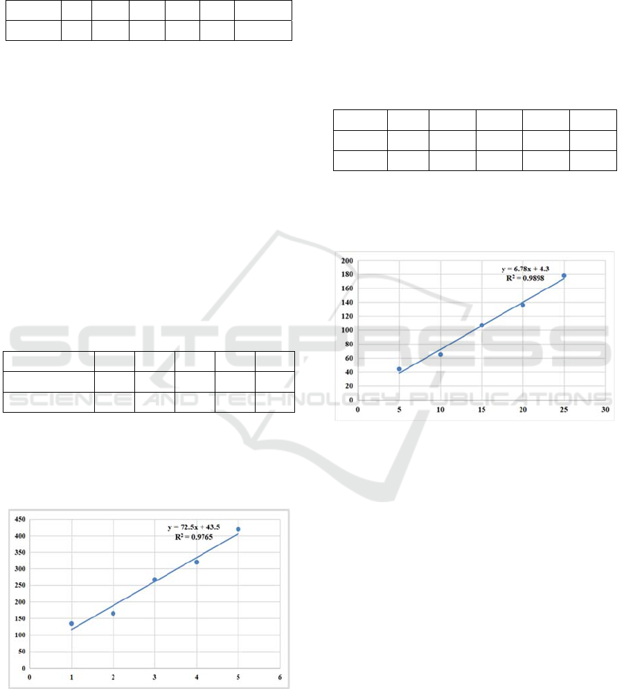
Table 8: Review, packaging, labeling and handling time
for different order quantities.
Test 1st 2n
d
3r
d
4th 5th
Total 1 2 3 4 5
Time(s) 79 163 202 289 350
Carry out linear regression fitting according to
the test results, as shown in Figure 5. Set the
intercept of the regression linear equation to zero,
and a
5
=71.218.
Research on Optimization of Stereoscopic Warehouse Delivery Mode Based on EIQ Analysis
79
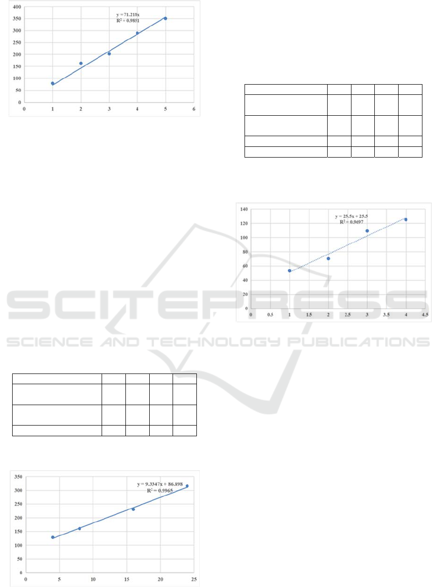
Figure 5: Fitting Chart of Review, Packaging, Labeling
and Handling Time.
mmaT 218.71
5
'
4
(12)
Wave sorting system time(T
5
')
The time for wave sorting of goods of the nth
item is t
5n
, which has the following relationship with
the shipment quantity CQ
n
and the shipment times
K
n
of the item:
6665
CKbCQat
nnn
(13)
In order to measure the values of a
6
, b
6
and c
6
,
using the control variable method, first set the
number of single product shipments K
n
as a fixed
value, change the value of single product shipments
CQ
n
, and add order information to test the single
product wave sorting time t
5n
in the virtual
simulation system. The test result data are shown in
Table 9.
Table 9: Control the number of shipments of single items,
wave sorting time.
Items I
1
I
2
I
3
I
4
frequency of Product
shi
p
ments
4 4 4 4
Quantity of Product
shi
p
ments
4 8 16 24
Time
(
s
)
128 160 230 315
Carry out linear regression fitting according to
the test data, as shown in Figure 6. a
6
=9.3347.
Figure 6: Fitting Chart of Controlling the Number of
Shipments of Single Items and Wave Sorting Time.
Set the single product shipment quantity CQ
n
as
a fixed value, change the value of single product
shipment times K
n
, and measure the single product
wave sorting time t
5n
. The test results are shown in
Table 10.
Table 10: Control shipment volume wave sorting time.
Items I
1
I
2
I
3
I
4
frequency of
Product shi
p
ments
1 2 3 4
Quantity of Product
shi
p
ments
4 4 4 4
Time
(
s
)
53 70 109 125
Carry out linear regression fitting according to
the test data, as shown in Figure 7. b
6
=25.5,
C
6
=25.5.
Figure 7: Fitting Chart of Wave Sorting Time for
Controlling Single Product Shipment.
)5.255.253347.9(
)(
666
5
'
5
KnCQ
cKbCQatT
n
nn
n
(14)
(3) Objective function formula
The shortest delivery time T of a batch order is
the shortest of the two delivery methods.
),min(
hd
TTT
(15)
By comparing the size of T
d
and T
h
, we can
determine which delivery method is more efficient,
and select the appropriate delivery method according
to the characteristics of the order.
3 INSPECTION OF DELIVERY
METHOD JUDGMENT MODEL
The judgment model of delivery mode is a
mathematical model based on the time
decomposition and summation of the operation
process and the simplification and abstraction of the
ICEMME 2022 - The International Conference on Economic Management and Model Engineering
80

actual operation process. The parameters of the
model are calculated based on the data obtained
from many experiments. In order to prove the
rationality and practicability of the model, the
correctness of the model is verified by substituting
the actual order information.
The system pre recorded four orders for EIQ
analysis, and the analysis results are shown in Table
11. The data obtained are substituted into the
delivery method judgment model.
Table 11: Statistics of EIQ data pre-recorded by the system.
m I
1
I
2
I
3
I
4
Q
m
N
m
1 2 2 2 5 11 4
2 3 2 0 6 11 3
3 1 0 4 6 11 3
4 3 1 2 5 11 4
CQ
n
10 5 9 22 Q N
K
n
4 3 3 4 44 14
(1) Delivery Time by Order (T
d
)
)(52.19635.22162.30211894.250
)2.86113.12()3.44478.6()45.43145.72(46.62
)2.863.12()3.478.6()5.435.72(6.62
4321
s
DQQmNm
TTTTT
m
d
(16)
(2) Consolidated order delivery time (T
h
)
)(39.87886.32201.18667.14885.220
)5.2545.25223347.9()5.2535.2593347.9(
)5.2535.2553347.9()5.2545.25103347.9(
)5.255.253347.9(
'
5
s
KnCQT
n
(17)
)(98.188239.87887.28462.3025.3336.83
39.8784218.71)3.44478.6()5.4345.72()8.6047.5(
218.71)3.478.6()5.435.72()8.607.5(
,
5
,
5
,
4
,
3
,
2
,
1
s
TmQmm
TTTTTT
h
(18)
It can be seen from the calculation results that
the delivery time Th of consolidated orders is
slightly less than the delivery time Td of orders, so it
is more efficient to select the delivery method of
consolidated orders.
The time calculated by the model is compared
with the data obtained from the actual experiment.
The comparison results are shown in Table 12.
Table 12: Time comparison table between the time
calculated by the four order models pre recorded by the
system and the actual time.
Model
calculation
Actual
measurement
error Error
rate
T
d
(s) 1963.52 1778 185.52 10.43%
T
h
(s) 1882.98 1638 244.98 14.95%
Although there is some difference between the
time spent in calculation and the actual operation,
about 10.43%, the result of using this model to
calculate the difference in delivery time is in line
with the actual situation.
4 CONCLUSIONS
In this paper, theoretical analysis and mathematical
modeling are closely linked when solving the issue
efficiency comparison problem between the
proposed issue by order method and the issue by
consolidated order method. With a large number of
specific data obtained through practical operation as
the theoretical basis, a discrimination model of
delivery mode based on EIQ analysis is established,
and the data is brought into the model for solution.
Qualitative analysis and quantitative calculation are
combined, and its effectiveness is confirmed through
verification.
REFERENCES
An Bin. Design and application of high-speed sorting
system simulation platform [D]. Shandong: Shandong
University, 2014.
Fan Qiyin. Research on sorting system of finished tobacco
distribution center [D]. Yunnan: Kunming University
of Technology, 2004.
Li Feng. Research on replenishment scheduling and
automatic sorting algorithm of tobacco distribution
center [D]. Hunan: Central South University, 2009.
Liu Jun. Application of EIQ Analysis Method in the
Planning of Cigarette Distribution Center [D]. Beijing
University of Posts and Telecommunications, 2010.
Liu Youquan. Application of EIQ Analysis Method in
Chain Operation Distribution Center and Case Study
[D]. Hubei: Huazhong University of Science and
Technology, 2005.
Research on Optimization of Stereoscopic Warehouse Delivery Mode Based on EIQ Analysis
81

Wei Xiaoqing. Application Research on Optimization of
Warehouse Location Operation Method of Finished
Product Warehouse in a Manufacturing Factory [D].
Shanghai: Shanghai Jiaotong University, 2013.
Wu Jing. Application of greedy algorithm based linear
programming in cargo location optimization [D].
Shanghai Jiaotong University, 2011.
ICEMME 2022 - The International Conference on Economic Management and Model Engineering
82
