Environmental Efficiency Assessment of the Chinese Industrial

Sector Considering Policymakers’ Preferences: A Two-Stage

Network SBM-DEA Approach

Junwei Sun

, Li Li and Peng Deng

School of Economics and Management, Harbin Institute of Technology, Shenzhen, China

Keywords: Environmental Efficiency, Two-Stage Network DEA, SBM Model, Policymakers’ Preferences.

Abstract: Efficiency improvements in the industrial sector are critical to the sustainable development of China’s

economy and the reduction of greenhouse gas (GHG) emissions. This paper extends the environmental

efficiency analysis from a “black box” to a network structure, where the industrial sector is divided into

industrial production and pollution treatment stages. Under the framework of cooperative game, a

slack-based two-stage network DEA model considering the preferences of policymakers is introduced and

the environmental efficiency of 30 provincial industrial sectors in China is evaluated for the period

2007-2015. The findings suggest that environmental efficiency is strongly influenced by policymakers’

preferences and exhibits divergent effects at the regional and provincial levels. Specifically, under either

weight distribution, the eastern region has the highest total efficiency, followed by the central and western

regions. Inter-regional efficiency differences are mainly due to differences in the pollution treatment stage.

At the provincial level, the heterogeneous effect of policymakers’ preferences can be grouped into four

categories. Finally, the level of coordinated development of industrial production and environmental

protection in China’s provinces is low, and the industrial green transformation needs to be continuously

promoted.

https://orcid.org/0000-0002-4650-9537

1 INTRODUCTION

Over the past decades, the industrial sector has

exhibited tremendous rapid growth and has become

the primary driving force of China’s economic

development. However, the industrial expansion

mode fueled by fossil energy has also brought about

unprecedented environmental degradation (Shao et

al. 2019). Moreover, as the world’s largest emitter of

GHG since 2006, China is under huge pressure to

reduce emissions worldwide, and the industrial

sector is the key to achieving these goals. Recently,

President Xi Jinping has officially announced that

China will spare no effort to reach peak carbon by

2030 and carbon neutrality by 2060. This task is

more challenging than expected because China is

still undergoing rapid industrialization and

urbanization, which means that the demand for

energy consumption will continue to increase for a

long time (Guo et al. 2021). Therefore, a more

suitable option for China is to improve

environmental efficiency through technological

progress and to reconcile economic growth with

environmental protection.

Generally, industrial system can be divided into

two interrelated stages, the production stage and the

treatment stage, respectively. Weighting methods for

subsystems are often used to capture the preferences

of policymakers. Specifically, a higher weighting of

the first stage implies that policymakers place more

importance on economic growth and vice versa for

environmental protection. Current studies usually

assume that policymakers give equal importance to

industrial production and pollution treatment, and

therefore adopt a simple equal-weight distribution

for the subsystem (Iftikhar et al. 2018). However,

the equal weight assignment ignores the potential

trade-off between economic growth and

environmental protection among regions, which is

inconsistent with practice and may yield misleading

results. Thus, this paper attempts to fill this gap and

Sun, J., Li, L. and Deng, P.

Environmental Efﬁciency Assessment of the Chinese Industrial Sector Considering Policymakers’ Preferences: A Two-Stage Network SBM-DEA Approach.

DOI: 10.5220/0012026100003620

In Proceedings of the 4th International Conference on Economic Management and Model Engineering (ICEMME 2022), pages 83-88

ISBN: 978-989-758-636-1

 2023 by SCITEPRESS – Science and Technology Publications, Lda. Under CC license (CC BY-NC-ND 4.0)

make contributions in the following aspects. Firstly,

a slack-based two-stage network model that

considers the internal structure is proposed to

provide more accurate results. Compared with

traditional CCR-based models, which assume

proportional changes in inputs or outputs, the

slack-based DEA model is non-radial and can

directly deal with input excess and output shortfall

(Tone and Tsutsui 2009). Secondly, this paper

attempts to set different weights for each stage to

examine the impact of various preferences of

policymakers on environmental efficiency.

The remainder of this paper is organized as

follows. Section 2 describes a slack-based two-stage

network DEA model based on the cooperative game

framework. The results and discussions are

presented in Section 3. Eventually, conclusions and

policy implications are provided.

2 METHODOLOGY

2.1 Slack-based Two-Stage Network

DEA Model

Suppose there are n DMUs, and in the first stage, the

observed data on the input, desirable output and

undesirable output vectors can be denoted as X

1,j

...X

i,j

...X

mp,j

) ≥0, Y

= (Y

1,j

...Y

i,j

...Y

sp,j

) ≥0 and

Z = (Z

1,j

...Z

i,j

...Z

h,j

) ≥0. The outputs Z generated in

the first stage are used as inputs for the second stage.

Besides, there’s an external input vector denoted by

= (X

1,j

...X

i,j

...X

mt,j

) putting into the pollution

treatment stage. The final product is represented by

= (Y

1,j

...Y

i,j

...Y

st,j

This paper builds on Iftikhar et al. (2018) by

assuming that all variables are freely disposable.

Besides, undesirable outputs in this paper are treated

directly as inputs based on Hailu and Veeman

(2001). All models presented in this paper are based

on the SBM method proposed by Tone (2001),

which has been widely used in many studies

associated with energy and environmental efficiency

measurements.

2.2 Environmental Efficiency

Measurement Based on the

Cooperative Game Framework

Referring to the seminal work of Liang et al. (2006),

the environmental efficiency of the two-stage

structure is calculated based on the cooperative

game framework. In this approach, the total

efficiency is first optimized, while the efficiency of

the subsystem is derived as a offspring from the

optimal solution that maximizes the efficiency of the

system. The model based on the SBM approach

under variable returns to scale (VRS) and free

linkage assumptions is as follows.

1k1 1 1

00 00

1( )1(+ )

min

p t

ptt

pzp tzt

iik

pik t ik

pro

ss ss

mxz mhxz

sy sy

−− −−

== ==



⋅− + + ⋅−







⋅+ + ⋅+





 



(1)

,1,...

, 1,...h

0, 1 1,...

0, 1,... 0, 1,... 0, 1,...h,

pp p p

jij i i p

pp p p

jrj r r p

jkj k k

ppzp

rpi pk

tt t

jij i i

xs xi m

ys yr s

zs zk

srssims k

st x s x

λλ

−

+− −

−

⋅+ = =

⋅==

⋅+ = =

≥==

≥= ≥= ≥=

⋅=

−



，，

，

, 1,...

, 1,...h

, 1,...

0, 1 1,...

0, 1,... 0, 1,... , 0, 1,...

0, 1,...h

jkj k k

pt t t

jrjr r t

itk rt

jkj jkj

zs zk

ys yr s

ims khs rs

zzk

λλ

−

−−+







⋅==

≥==

≥= ≥ = ≥ =

⋅⋅==

−





，





(2)

Where

−

and

−

are slacks of inputs,

outputs, and undesirable outputs in production stage,

respectively.

−

and

−

are slacks of inputs,

intermediate variables, and undesirable outputs in

treatment stage, respectively. Besides,

and

are

intensity variable for production and treatment stage,

respectively.

and

are the weights of individual

stages with respect to its importance, which satisfy

the constraints:

ww=

. Based on the total

efficiency, the production efficiency and the

treatment efficiency can be defined as

and

The efficiency of production stage:

(

pik

mxz

−−



−+







(3)

The efficiency of treatment stage:

ICEMME 2022 - The International Conference on Economic Management and Model Engineering

1( )

)

tik

mxz

−−

−

 + 



(4)

2.3 Variables and Data

2.3.1 Input-Output Variables

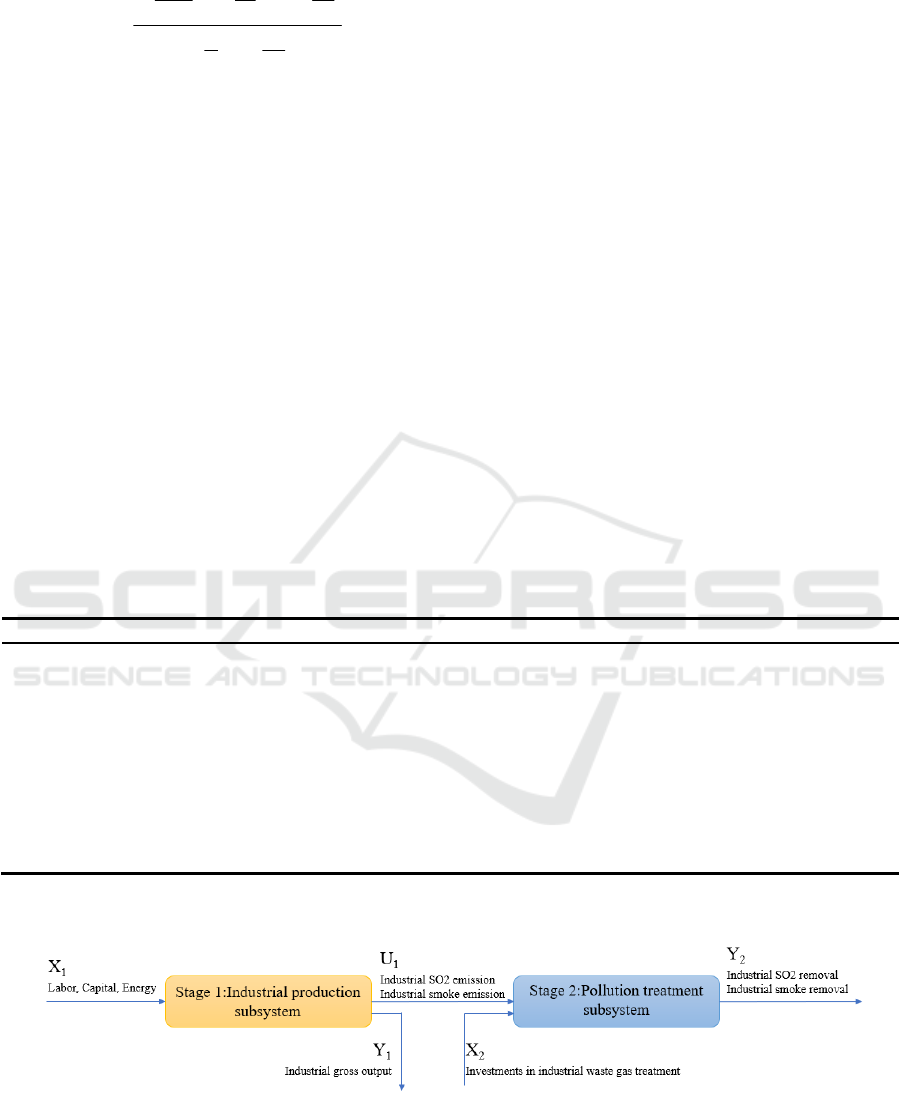
Figure 1 illustrates the operational mechanism of the

two-stage network DEA model for industrial system.

denotes the input variables of industrial

production, including labor, capital, and energy. The

desirable output produced in this stage is represented

by Y

, while undesirable outputs are represented by

. The efficiency of this sub-stage is called total

factor productivity (PE). These undesirable outputs

from the first stage are also inputs to the second

stage and are referred to as intermediate products. In

the pollution treatment stage, intermediate products

and exogenous inputs represented by X

are

converted to desirable outputs represented by Y

The efficiency of this sub-stage is called the

pollution treatment efficiency (TE). The total

efficiency is calculated by considering these two

stages and is called environmental efficiency (EE).

Based on data availability, this paper uses data

from 2007-2015 for 30 Chinese provinces (except

Hong Kong, Macao, Taiwan and Tibet) to measure

environmental efficiency. The three inputs to the

industrial production subsystem are labor, capital,

and energy. Labor is calculated by the average

number of industrial employees per year. Capital is

estimated using the Perpetual Inventory Method

(PIM). Energy is measured as total energy

consumption, all of which is converted to 10,000

tons of coal equivalent (tce). Gross industrial output

is chosen as a proxy for desirable output and

deflated by the Producer Price Index (PPI) in

constant 2003 prices. The undesirable outputs are

industrial SO

and smoke emissions, which represent

emissions from industrial processes that are not

treated in any way. In the second stage, the inputs

consist of two components: first, exogenous inputs,

such as investments in industrial waste gas

treatment; and second, undesirable outputs generated

in the first stage. The desirable outputs are SO

removal and smoke removal, indicating the

effectiveness of the pollution treatment. The

variables are described in detail in Table 1.

Table 1: Description of the variables.

Variables Unit Data source

Industrial

roduction subs

stem

Input(X

) Labor

Capital

Energ

Ten thousand

Hundred million

Ten thousand tce

CSY

CESY

Desirable out

(

)

Gross industrial out

ut Hundred million CIESY

Undesirable output(U

)

(Intermediate output)

Industrial SO

emission

Industrial smoke emission

Ten thousand tons

CSY, CEY, CCSY

CSY, CEY

Pollution treatment subs

stem

Input(X

) Investments in industrial waste gas treatment Hundred million CESY

Desirable output (Y

) Industrial SO

removal

Industrial smoke removal

Ten thousand tons

CSY, CCSY

CSY, CEY, CCSY

Note: CSY denotes China Statistical Yearbook; CEY denotes China Environmental Yearbook; CESY denotes China Energy

Statistical Yearbook; CIESY denotes China Industry Economy Statistical Yearbook; CCSY denotes China City Statistical

Yearbook; CESY denotes China Environmental Statistics Yearbook.

Figure 1: Two-stage system of industrial production and environmental treatment.

2.3.2 Sub-Stage Weight Indicator

Referring to Bian et al. (2015), this paper uses the

ratio of energy conservation and environmental

protection expenditure to total fiscal expenditure to

capture policymakers’ preferences. Specifically, let

Environmental Efﬁciency Assessment of the Chinese Industrial Sector Considering Policymakers’ Preferences: A Two-Stage Network

SBM-DEA Approach

E denote the annual amount of regional spending on

energy conservation and environmental protection,

and P denote the amount of regional spending to

support production and construction. Thus, W

P/(E+P), and accordingly W

= 1- W

. The results

show that the weights assigned by local governments

to the production and treatment stages are relatively

stable from 2007 to 2015, with W

ranging from

0.876 to 0.898 and W

ranging from 0.102 to 0.124.

The sub-stage weight indicator is described in detail

in Table 2.

Table 2: The sub-stage weight indicator.

2007 2008 2009 2010 2011 2012 2013 2014 2015

0.880 0.876 0.880 0.876 0.898 0.896 0.894 0.897 0.893

Wt 0.120 0.124 0.120 0.124 0.102 0.104 0.106 0.103 0.107

3 RESULTS AND DISCUSSIONS

3.1 The Impact of Policymakers’

Preferences on Environmental

Efficiency

3.1.1 Regional Heterogeneity Analysis

Referring to Wu et al. (2016), policymakers’

preferences are distinguished by the weights

assigned to each subsystem, and simply assume that

is between 0.1 and 0.9. As shown in Table 3, the

total efficiency (EE) keeps increasing from 0.673 to

0.738 with the increase of W

, and the pollution

treatment efficiency (TE) is also on the rise with a

growth rate of approximately 37.97%, which far

exceeds the growth of EE. Total factor efficiency

(PE), on the other hand, shows the opposite

direction. Notably, there is an inflection point in the

contribution of sub-stages to the total efficiency,

with TE becoming the primary driver of EE when

>0.6. This finding suggests that environmental

efficiency is strongly affected by policymakers’

preferences. In addition, significant regional

differences are found in the impact of policymakers’

preferences. Under either weight distribution, the

eastern region has the highest environmental

efficiency, followed by the central and western

regions. The differences in total efficiency between

regions are mainly due to differences in the

efficiency of the treatment stages.

Table 3: The impact of policymakers’ preferences on environmental efficiency.

ion

0.1 0.2 0.3 0.4 0.5 0.6 0.7 0.8 0.9

East

EE 0.757 0.759 0.760 0.762 0.763 0.765 0.766 0.768 0.771

PE 0.975 0.951 0.928 0.901 0.876 0.852 0.831 0.810 0.791

TE 0.773 0.791 0.810 0.832 0.856 0.883 0.909 0.939 0.969

Central

EE 0.630 0.637 0.645 0.655 0.665 0.677 0.690 0.706 0.724

PE 0.973 0.947 0.920 0.894 0.864 0.839 0.814 0.790 0.766

TE 0.646 0.672 0.699 0.729 0.767 0.802 0.843 0.889 0.942

West

EE 0.620 0.626 0.634 0.644 0.655 0.667 0.681 0.698 0.717

PE 0.970 0.939 0.910 0.880 0.853 0.828 0.804 0.781 0.758

TE 0.638 0.664 0.692 0.725 0.759 0.798 0.839 0.888 0.942

Total

Sample

EE 0.673 0.677 0.683 0.690 0.697 0.705 0.715 0.726 0.738

PE 0.973 0.945 0.919 0.891 0.865 0.839 0.816 0.794 0.772

TE 0.690 0.712 0.737 0.765 0.797 0.830 0.866 0.907 0.952

Note: EE denotes overall efficiency, PE denotes total factor efficiency, TE denotes pollution treatment efficiency.

3.1.2 Provincial Heterogeneity Analysis

Heterogeneous effects of policymakers’ preferences

on provincial environmental efficiency can be

classified into four categories. The first category

indicates that the efficiency is not influenced by

policymakers’ preferences, such as Beijing, Jiangsu,

Jiangxi, Shandong, Guangdong, Hainan, and Gansu.

The second category refers to the fact that the more

priority is given to production stage, the lower the

total efficiency. That is, in order to maximize total

efficiency, more emphasis needs to be placed on

pollution control rather than industrial production.

The third category indicates that total efficiency

ICEMME 2022 - The International Conference on Economic Management and Model Engineering

increases with higher production weights, suggesting

the need to focus on the production side to increase

green total factor productivity. The last category

demonstrates that there is a turning point in the

effect of policymakers’ preferences, exhibiting an

inverted U-shaped trend. The total efficiency rises

first with the increase of W

, and then decreases after

reaching the turning point. The efficiency of such

provinces peaks in a given combination of weights.

For instance, the optimal combination of weights for

and W

in Tianjin in 2015 is (0.8,0.2). Similarly,

the combination for Shanghai in 2015 is (0.8,0.2),

Hubei is (0.2,0.8), and Guizhou is (0.6,0.4).

3.2 Evaluation of the Coordination of

Industrial Development

This section uses the sub-stage weight indicators in

subsection 2.3.2 to calculate the environmental

efficiency of the industrial sector in each province of

China from 2007-2015. The relative ranking of

environmental efficiency is used to represent the

degree of coordinated industrial development in

each province. All provinces are divided into four

categories based on their ranking, such as highly

coordinated, moderately coordinated, uncoordinated

and highly uncoordinated. To capture the dynamic

trend, we further divide the period into 2007-2010

and 2012-2015; the former belongs to the 11th

Five-Year Plan and the latter belongs to the 12th

Five-Year Plan. As shown in Table 4, China’s

provinces have a relatively low level of industrial

coordination development, with a deteriorating trend

during the 12th Five-Year Plan. Nearly half of the

provinces face a critical imbalance between

industrial development and environmental

protection, most of which are central and western

provinces. Only six provinces, including Beijing,

Shandong, Jiangxi, Guangdong, Hainan, and

Shanghai, have achieved coordinated development

of industrial production and environmental

protection, while Xinjiang, Sichuan, and Liaoning

continue to suffer from a mismatch between

industrial production and pollution control. In

contrast, provinces such as Henan, Jiangsu, Hunan,

Tianjin, Hubei and Yunnan have made great

progress in the coordinated development of

production and environmental protection.

Table 4: The level of coordinated industrial development in China’s provinces.

East

2015