
The Best Decision-Making Scheme Based on Bitcoin and Gold Stock
Market
Jingru Zeng, Yufei Wang
*
and Xiyu Zheng
International College Wuhan University of Science and Technology, Wuhan, China
Keywords: Unstable Assets, Bull and Bear Market Judgment Model, Risk Model, Time Series Prediction Model, Xgboost
Regression Model.
Abstract: Market traders frequently buy or sell their volatile assets, Bitcoin and gold, in order to maximize their returns,
and each purchase and sale of these two assets requires a commission. In order to study this economic
management problem, we made certain assumptions and established a prediction model to achieve the best
rete of returns. We construct bull and bear market judgment models, risk models and time series prediction
models to help traders make the best decisions every day in order to maximize profits. Find the total assets in
the hands of traders as of 9/10/2021. To demonstrate the feasibility of our strategy, we use XGboost regression
model to fit the predicted data and the real data. After determining the sensitivity of the model and analyzing
the impact of market price fluctuations on our model, we communicated our decisions, models, and results to
traders in the form of memos. In summary, when you have $1000 on September 11, 2016, through our model
based on five years’ market data, you will have $184659.88 on September 10, 2021.
1 INTRODUCTION
Market traders often buy or sell their volatile assets -
bitcoin and gold - to maximize their returns. Each
purchase or sale of these two assets requires a
commission, and while gold is not open every day,
bitcoin can be bought and sold daily. The trader would
have a principal of $1,000 on November 9, 2016, and
would use that money to invest and trade gold and
bitcoin over a five-year period from November 9,
2016, to September 10, 2021, to maximize their
returns. We categorize this problem as a quantitative
economic investment strategy analysis problem
(Tang, 2021), quantitative investment is a type of
trading with quantitative statistical analysis tools at its
core and programmed trading (Guo, 2014; Hou,
2021). We use data from the past five days to predict
the future day's gold and bitcoin prices and build a
dynamic programming model to determine the
objective function (Gou, 2022). Specifically, our
work starts with data preprocessing of the trading
market amounts for the last five years of trading, and
since traders cannot determine the market stock
movements for the day after, we form our total model
*
Corresponding author
part by building three models: a bull and bear market
model, a risk forecasting model and a time series
forecasting model. It is used to forecast the economic
conditions of the market stocks on a 5-day basis. This
model is used to determine daily trading decisions
and to calculate total assets on hand on 10/9/21. Next
is to use our regression model using machine learning
XGboost to learn all the transaction amounts over the
five years and fit them to the data obtained from our
model to test the accuracy of the decision model.
Finally starting with the commission collection for
each trade, we determine the sensitivity of the trade
and analyze the impact of price fluctuations on us.
2 RELATED WORK
As we provide traders with a daily decision-making
solution, it is important to forecast the direction of the
market. It is difficult to predict the trend of the stock
market because of the many factors and complex
relationships that influence it. In this regard, we have
made progress in understanding the development of a
good prediction model by consulting the literature on
338
Zeng, J., Wang, Y. and Zheng, X.
The Best Decision-Making Scheme Based on Bitcoin and Gold Stock Market.
DOI: 10.5220/0012030400003620
In Proceedings of the 4th International Conference on Economic Management and Model Engineering (ICEMME 2022), pages 338-344
ISBN: 978-989-758-636-1
Copyright
c
2023 by SCITEPRESS – Science and Technology Publications, Lda. Under CC license (CC BY-NC-ND 4.0)

stock market prediction models. Based on the neural
network integration theory, we developed a stock
market forecasting model. The "Basic Data Model",
"Technical Indicator Model" and "Macro Analysis
Model" were developed and finally a simple average
was used to create an integrated system (Zhang,
2003). The corresponding BP algorithm network
forecasting model and ARCH (1) and GARCH (1,1)
forecasting models are also developed to forecast the
volatility of the closing price of the Shenzhen Stock
Index at each weekend using the actual data of the
Shenzhen stock market in China (Pang, 2006). In
addition, a stock-specific forecasting estimation
method is proposed based on a specific state space
form consisting of a combination of trend, smooth
autoregressive and nonlinear heteroscedastic random
variables (Wang, 2010). Drawing on the advantages
of spatial reconstruction techniques and visual data
analysis techniques for expressing the patterns and
characteristics of complex systems, graphical
methods for forecasting stock market trends based on
minute-by-minute stock market trading information
have been proposed (Hu, 2014). A stock-specific
forecasting estimation method is proposed based on a
specific state space form consisting of a combination
of trend, smooth autoregressive and nonlinear
heteroskedastic random variables (Zhu, 2006). The
new XGBoost-ARIMA hybrid forecasting model is
also suitable for forecasting about daily average data
(Liu, 2022).
In order to optimize various forecasting
models, the Realized GARCH model is a good
choice. In addition, the study ignores the impact of
the information contained in the exchange volume on
the stock price volatility, which may lead to biased
estimation of the model parameters. Stochastic
volatility models based on Poisson distribution can
not only effectively solve the problem of
underutilization of volume information by traditional
practices (Sun, 2019). The analysis and judgment of
the stock market is also crucial to the proposed
decision. Using parametric and semiparametric
methods, we judge and predict the bull and bear
market cycles of the stock market (Ye, 2021). In the
case that short selling is not allowed, a log-optimal
portfolio model with conditional value-at-risk as the
risk measure can be established based on the
conditional value-at-risk proposed by Rockefeller
(Moazeni, 2015). In order to optimize various
forecasting models, the Realized GARCH model is a
good choice. In addition, the study ignores the impact
of the information contained in the exchange volume
on the stock price volatility, which may lead to biased
estimation of the model parameters (Shi, 2019).
A
new multifractal volatility forecasting model was
constructed based on the HAR model, taking into
account the intra-day effects of high frequency stock
market data and the measurement error of realized
volatility to revise the existing multifractal volatility
indicator construction method. The models were
evaluated using the Diebold-Mariano test and the
"model confidence setting" test (Yuan, 2020).
3 EXPERIMENT
According to the daily price of gold and bitcoin in the
past five years, this method forecasts the price of gold
and bitcoin in a certain period of time, and finally
makes the most profitable measure according to the
assumption of bull and bear market. From the table,
we find that the prices of gold and bitcoin are
increasing in the general situation, and the prices
themselves are related to the prices of the previous
year; In the short term, it will be affected by the local
market policies and other uncertain factors and will
increase or decrease. According to the above two
characteristics, we choose to use AR autoregressive
model to simulate and forecast the amount of money
we need in the time period according to the known
data. First of all, we need to test the data to see if they
are stable, if not, then we need to make small changes
and debug them until the conditions are met. We use
the method called Daniel test, which is mainly around
the Spearman correlation coefficient. Spearman
correlation coefficient 𝑞
and statistical
variables 𝑇 The formula is as follows:
𝑞
=1−
(
)
(
𝑡−𝑅
)
(1)
𝑇=
√
(2)
After knowing the above two quantities, we can
start the test.
For a set of data, there will be the rank of the time
series (sort the data from small to large, and the rank
of each data is its serial number). We use MATLAB's
own algorithm to calculate the rank of the data.𝑅𝑡 ;
For significant levels𝛼From the time series (the
matrix of data in the file), calculate (t_0, 𝑅𝑡 ), t_0 =
1,2, …, the correlation coefficient of n. If | T | ≤ t_0,
then the sequence is stationary; Conversely, if | T | ≥
t_0, it is not stationary and 𝑞𝑠 > 0, showing an upward
trend. The specific operation is shown below:
clc, clear;
[a]=xlsread('BCHAIN-MKPRU','B3:B1827');
a=a';
Rt=tiedrank(a);
n=length(a); t=1:n;
The Best Decision-Making Scheme Based on Bitcoin and Gold Stock Market
339

Qs=1-6/n*(n^2-1)*sum((t-Rt).^2);
T=Qs*sqrt(n-2)/sqrt(1-Qs^2);
t_0=tinv(0.995,n-2);
To debug data, we take to do the first-order
difference operation, that is, the new sequence 𝑏
=
𝑎
−𝑎
, then you can easily get 𝑎
=𝑏
+𝑎
,
and here a𝑎
is the prediction value we calculated,
𝑏
is the new sequence we will 𝑎
for change to get,
that is, to meet the use of smooth time series
conditions of the sequence, here We subject the new
series to another Daniel's test.
b=diff(a);
[Tb,t_00]=spearman(b);
The Spearman function is the function that we
check whether the sequence is stationary. To put it
simply, we will summarize our previous work and see
them written into a new function.
function [T,t_0]=spearman(a)
a=a'; a=a(:); a=a';
Rt=tieddrank(a);
n=length(a); t=1:n;
Qs=1-6/n*(n^2-1)*sum((t-Rt).^2);
T=Qs*sqrt(n-2)/sqrt(1-Qs^2);
t_0=tinv(0.995,n-2);
The debugged data is the precondition of AR
autoregressive model. At this time, we put the
debugged data into the model.
According to the theory, we know that the formula
of AR autoregressive model is as follows:
𝑦
=𝑐
𝑦
+𝑐
𝑦
+⋯+𝑐
𝑦
+𝜀
(3)
It can be clearly seen that the regression equation
𝑦
is composed of the first p terms and the last 𝜀
(i.e.,
the random perturbation term with a mean of 0), and
the theory of this AR autoregressive model is that the
data of the t
th
year is expressed with the data of the
previous p years, and finally the AR(p) is formed, and
this p, we use the AIC criterion to seek, and finally
our p = 6, as follows.
m=ar(b,6,'1s');
bhat=predict(m,[b';1000:]);
ahat=[a(1),a+bhat'];
delat=abs((ahat(end-1)-a)./a);
There are several unknown representations above:
m is a vector composed of c_1, c_2, ..., will find him,
we can get to the expression of the function AR (p),
the completion of the expression will mean that we
can find the new sequence b, and then we will
calculate the ahat (the first few fitted values and the
n+1 predicted value, the first fitted value may have a
difference with the But the final delat is the algorithm
for calculating the relative error, where our relative
error is very small, probably only about 0.00008), and
the final result is our predicted value.
We need to judge whether it is the best way to
judge whether it is the best way to make a profit by
buying or selling gold in the bull market or in the bull
market every day. After making this judgment,
according to the price of the previous few days, judge
whether to trade on the same day. The specific
judgment methods of the model are as follows.
We assume that if the average amount of the
current cycle is higher than 20% of the previous
cycle, it is considered as a "bull market", and we will
sell it in full. Assuming that the average amount in the
current cycle is less than 80% of the previous cycle,
we consider it a "bear market" and we will buy gold
or bitcoin. Based on the average amount of each
period obtained from the previous data analysis,
Establish the judgment model of "bear market" and
"bull market" in each cycle.
NUM=xlsread('C:\Users\wyf\Documents\
WeChat Files\wxid_uknuh3yjrrhv22\
File\2022-
02\333.xlsx');
a=NUM'
a=round(a);
disp(a);
for ii=2:length(a)
if a(1,ii)>=1.05*a(1,ii-1)
disp('This was the bull market.')
elseif a(1,ii-1)*0.95>=a(1,ii)
disp('This was the bull market.')
else
continue
end
end
Second, we need to judge whether traders will
buy, hold or sell gold and bitcoin on a certain day.
Here, we simply use MATLAB to realize our
hypothesis. First of all, let's assume that a certain day
is an unknown day in the 21
st
century, then we input
the number into MATLAB and bring it into the code.
We can get the conclusion that a = 1\0\2.
Assuming that the date we input is September 20,
2017, we can clearly see that this day is the 368
th
day
from September 12, 2016, and the final conclusion is
a = 0 (buy). We use the data given in the title and
further optimize it to form a new table and bring it
into MATLAB. The specific operation code is shown
in the following:
clc, clear;
y=input('input years:');
m=input('input months:');
t=input('input dates:');
date=(y-2016)*360+(m-9)*30+(t-12);
[NUM]=xlsread('BCHAIN-MKPRU',1);
b=NUM(date-4:date);
ave=mean(v)
ICEMME 2022 - The International Conference on Economic Management and Model Engineering
340

if b-ave>=0.2*ave
a=1;
elseif ave-b>=0.2*ave
a=0;
else
a=2;
end
4 RESULTS AND EVALUATION
In this section, we will show the results of our model.
The first is our data detection results. If the two Excel
data mentioned above are not stable, AR
autoregression is not possible. According to the
programming results, |T| ≥ t_0, and 𝑞
>
0.Therefore, we have verified our previous idea that
it is unstable, so our later step is to make the data
stable, and then run the AR autoregressive model.
Secondly, we put the above debugged data into the
programming system of AR model. In the middle, we
interspersed the verification that the debugged data is
stable. Taking bitcoin as an example, its result is t =
0.000000 million+42.696604080418390i, t_0 =
2.578528918212297, which obviously satisfies |T| ≤
t_0. Therefore, the new sequence B created is the
data sequence satisfying AR autoregressive model.
Finally, sequence B is brought into the MATLAB
programming function of AR autoregressive model.
The result is that the price of bitcoin on September
10, 2021 is $46161, while the price of gold is
$1796.5.
Finally, the most important result is the result of
solving the problem. While judging the bull and bear
market, we combine the results of each cycle with the
price of gold bitcoin to calculate the final profit we
get. Here we start with three assumptions about how
to allocate the $1000.
4.1 Suppose You Cost All $1000 for
Gold
Purchase price: $1324.6
Selling price (assuming last day sell): $1796.5
Ultimate Assets: $1356.3
4.2 Suppose You Cost All $1000 for
Bitcoin
Purchase price: $621.65
Selling price (assuming last day sell): $ 46161
Ultimate Assets: $74255.6
4.3 Suppose You Cost $500 for Gold
and $500 for Bitcoin
Bitcoin purchase price: $621.65
Bitcoin selling price (assuming last day): $46161
Gold buying price: $1324.6
Gold selling price (assuming last day): $1796.5
Ultimate Assets: $86734.7
We decided to start the investment plan in the
form of 50% investment, that is, half of the money to
buy gold, half of the money to buy bitcoin. In this
way, we can get the most cost, which is our best
trading plan.
We choose to put the average bitcoin price of the
previous five-day line and the average price of gold
on the 15th day line into MATLAB for analysis.
Using the code of "the price of the day and the
judgment of the previous cycle", we classify the
needs of buying, selling and holding, and then further
calculate and distribute the money in proportion. The
specific operation is as follows:
[NUM]=xlsread('liangbaihebing(1)',1,'C2:C1827'
);
NUM(isnan(NUM(:,1))==1)=[];
NUM=NUM';
A=A';
l=length(NUM);
i=1;
while(i<=1)
if NUM(i)-NUM(i+1)>=0.1*NUM(i)
a=1;i=i+1;
elseif NUM(i+1)-NUM(i)>=0.1*NUM(i+1)
a=0:i=i+1;
else
a=2;i=i+1;
end
A(i)=a;
end
According to the above method, the final result is:
from September 10, 2016 to September 10, 2021, the
final amount is $184659.88.
In the previous model part, we established AR
autoregressive model to predict the future stock price
trend of bitcoin and gold. Through the establishment
of risk model and bull bear market model, we got our
best plan. In order to prove the feasibility of the
strategy, it is necessary to test the fitting degree
between the time series prediction and the reality.
With the return of XGboost, we simulated the trend
of bitcoin and gold and compared it with the actual
situation.
Since the amount of data is too large (more than
1000 lines), and the results of each simulation will
change due to the debugging of simulation parameters
The Best Decision-Making Scheme Based on Bitcoin and Gold Stock Market
341
of XGboost regression, we consider the operation of
the program, that is, bitcoin is divided into two parts
by 5/31/19, that is, the first 993 days and the last 833
days. Gold is divided into the first 1000 days and the
last 266 days by 8/24/20.
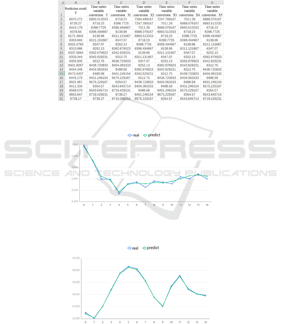
The first analysis is the two parts of Bitcoin. First,
we can see the first 993 days, as shown in the Figure
below, which is the quantitative Y of time series
analysis and some data of X1, X2, X3, X4 and X5
(due to the large number of data, we can’t show them
one by one).
Figure 1: XGboost model testing data (partial).
Then the regression simulation of 993 before
Bitcoin is:
Figure 2: First 993 days for Bitcoin.
Using the same analysis method, we also get the
fit between the predicted value and the actual value of
the second half of Bitcoin:
Figure 3: The last 833 days for Bitcoin.
ICEMME 2022 - The International Conference on Economic Management and Model Engineering
342
Through this fitting, we can clearly see that
although there is a slight deviation in the first half of
the forecast trend, it will not be very serious. The error
range is controlled around 100, which has no obvious
impact on our final results. The second half of the
simulation is perfect, which shows that our timing
forecast is very suitable for the market trend of
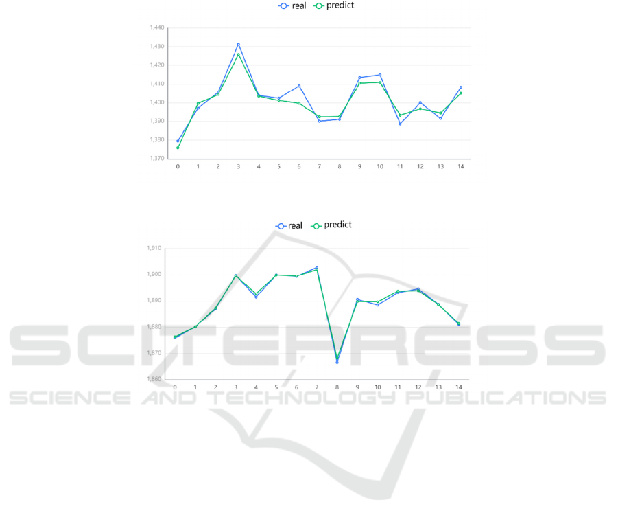
Bitcoin. The next step is the simulation of gold. The
simulation of gold is as Fig.3 and Fig.4.
Figure 4: First 993 days for gold.
Figure 5: The last 833 days for gold.
As can be seen from the two fitting curves in the
above chart, although there are some deviations in the
trend prediction of the first half of gold, the maximum
value is not more than 10. Combined with the
simulation of the second half, it can be said that our
simulation results are very impressive. To sum up, our
decision-making model is very precise and
reasonable.
5 DISCUSSION AND
CONCLUSION
Based on the data of gold and bitcoin trading markets
in the past five years, we have constructed the
judgment model, risk model and time series
prediction model of bull and bear markets to help
traders make the best decisions every day in five
years, so as to maximize profits. From September 10,
2016 to September 9, 2021, the total assets held by
traders increased from $1000 to $184659. At the same
time, XGboost regression model is used to fit the
predicted data and the real data, and the better fitting
results are obtained. The advantages of our decision-
making are obvious. The three models
comprehensively analyze the fluctuation of stock
market price. When verifying the fitting degree of
time series prediction, we choose XGboost to fit to
achieve better results. But unfortunately, the risk
indicators in the model still need to be considered
comprehensively. In a word, our decision-making
model provides a good reference for traders' decision-
making.
REFERENCES
Guo Xicai. The development and supervision of
quantitative investment[J]. Jiangxi Social Sciences, vol.
3, pp. 58-62, 2014.
Hou Xiaohui, Wang Bo. Quantitative investment based on
fundamental analysis: Research Review and
The Best Decision-Making Scheme Based on Bitcoin and Gold Stock Market
343

prospect[J]. Journal of Northeast Normal University,
vol. 3, pp. 124-131, 2021.
Hu Min, Sun Yufeng. Visual prediction of stock market
trend based on state evolution[J]. Journal of computer
aided design and graphics, vol. 02, pp. 302-313, 2014.
Liu Yongmin, Luo Haoyi, Xie Tieqiang. PM based on
XGboost Arima method_(2.5) research and application
of mass concentration prediction model[J]. Journal of
safety and environment, vol.3, pp. 1-13, 2022.
Moazeni S, Powell W B, Hajimiragha A H. Mean-
Conditional Value-at-Risk Optimal Energy Storage
Operation in the Presence of Transaction Costs[J].
IEEE Transactions on Power Systems, vol. 30(3), pp.
1222-1232, 2015.
Pang Sulin, Xu Jianmin, Li Rong. The empirical
comparison of BP algorithm and symmetric arch model
for Stock Market Volatility Prediction[J]. Control
theory and response, vol. 04, pp. 658-662, 2006.
Shi Yanlin, AI Chunrong. The intra week characteristics of
volatility in China’s stock market and its prediction
model[J]. System theory and practice, vol. 04, pp. 935-
945, 2019.
Sun Yanlin, Chen Shoudong, Liu Yang, Stock Price
Volatility Prediction Based on stock market and foreign
exchange volume information[J]. System theory and
practice, vol. 04, pp. 935-945, 2019.
Wang Wenbo, Fei Fusheng, Yi Xuming. Prediction of
China's stock market based on EMD and neural
network[J]. System theory and practice, vol. 06, pp.
1027-1033, 2010.
Xianwei Gou. Analysis of Quantitative Economic
Investment Strategy[J]. Scientific Journal of Intelligent
Systems Research, vol. 4(4), pp.34-54, 2022.
Ye Lu, Wang Zhizheng. Identification and prediction of bull
and bear market in Chinese stock market [J] Statistics
and decision making, vol. 37(20), pp. 161-165, 2021.
Yuan Ying, Chen Shoudong, Liu Xin. Research on
multifractal modeling and prediction of China’s stock
market [J]. System theory and practice, vol. 09, pp.
2269-2281, 2020.
Zihe Tang and Yanqi Cheng and Ziyao Wang. Quantified
Investment Strategies and Excess Returns: Stock Price
Forecasting Based on Machine Learning[J]. Academic
Journal of Computing & Information Science, vol. 4,
pp.24-34,2021.
Zhang Xiuyan, Xu Benben. Stock market forecasting model
based on neural network integrated system[J]. System
theory and practice, vol. 09, pp. 67-70, 2003.
Zhu Yu, Shi Zhongke. The spatial trend method of stock
market[M], vol. 05, 2006, pp. 567-570.
ICEMME 2022 - The International Conference on Economic Management and Model Engineering
344
