
Option Pricing and Risk Hedging in Current Financial Market:
A Case for Pfizer
Hang Zhang
Liberal Arts & Sciences, University of Connecticut, l22 Eastwood Rd, Storrs, CT, 06268, U.S.A.
Keywords: BS, BT, Option Pricing, Pfizer.
Abstract: The research background of this paper is that in stock option trading, the risk is weakened, and the profit
level is improved by means of hedging. This paper discusses and analyzes the differences in the hedging
results of stock options of the same company based on different option pricing models. The data adopts the
stock option trading data of Pfizer, and uses the historical data model, BS (black-Scholes) model, and BT
(Binomial Tree) model to construct an option pricing model and calibrate it, and finally perform delta
hedging. The results show that the historical data model shows the best results in the final hedging, the
hedging results of the BS model are in the middle level, while the hedging results of the BT model are not
satisfactory in this study. This research appears in stock option trading, and the investment behavior of
single company stock option as the target weakens the comprehensive risk and improves the comprehensive
profit level.
1 INTRODUCTION
Beginning in the second half of 2019, Covid-19
spread recklessly around the world, which has
brought huge negative impact on people's daily life
and production and construction. With the
development and production of vaccines and antiviral
drugs, people are working hard to fight and defeat the
virus. In this process, pharmaceutical companies
have become bridgeheads to overcome difficulties,
and have introduced a large amount of funds for
scientific research and development and drug
production. Therefore, in the post-epidemic era,
companies in the field of big health are generally
beneficial. As one of the top pharmaceutical
companies, Pfizer has become the most favored
company by investors in the pharmaceutical industry.
However, with the influx of more and more
investors, the phenomenon of blind investment and
follow-up buying continues to appear. People are
superstitious about the long-term benefits of the
pharmaceutical industry, while ignoring the objective
risks in stock option trading. Therefore, it is very
important to choose a suitable option pricing model
and a reasonable hedging strategy, which will help to
reduce risks and improve returns.
The research on stock option pricing model and
hedging strategy is not a new topic in the industry.
Around this center, in the current field, many
scholars have expressed their views on option pricing
models and their understanding of hedging strategies.
Li Xu, Shijie Deng, Valerie M. Thomas co-published
article and hold the idea that options that the impact
of market volatility on option prices is divided into
effectiveness and destructiveness (Xu, 2016).
Ghulam Sarwar wrote that there is contemporaneous
positive feedback between the volatility of the
exchange rate and the trading volume of call and put
options (Sarwar, 2003). The paper completed by Jie
cao and Bing Han pointed out that when using delta
to hedge stock options, as the heterogeneous
volatility of the underlying stock increases, returns
show a monotonically decreasing trend (Cao, 2013).
Research by Gurdip Bakshi and Nikunj Kapadia
found that delta-hedged portfolio returns are
correlated with changes in the volatility risk premium
(Bakshi, 2003). When Erik Ekström and Johan Tysk
studied stochastic volatility and the Black-Scholes
equation, they found that option prices are the only
classical solution to parabolic differential equations,
and this solution is bounded (Ekström, 2010). Yisong
Tian's research pointed out that the calibrated
binomial model can recalibrate the binary tree
through the skew parameter, this method allows the
Zhang, H.
Option Pricing and Risk Hedging in Current Financial Market: A Case for Pfizer.
DOI: 10.5220/0012033400003620
In Proceedings of the 4th International Conference on Economic Management and Model Engineering (ICEMME 2022), pages 381-386
ISBN: 978-989-758-636-1
Copyright
c
2023 by SCITEPRESS – Science and Technology Publications, Lda. Under CC license (CC BY-NC-ND 4.0)
381
location of barrier location nodes based on different
option form prices (Tian, 1999).
The propositions and findings of the above
scholars are worth studying and learning. On this
basis, this paper sets the research focus on the
differences in the performance of hedging strategies
based on different option pricing models when
investing in stock options of the same company.
Taking Pfizer's stock option positioning data as the
object, using historical data model, Black-Scholes
model and Binomial Tree model to construct and
calibrate three different option pricing models, and
then perform hedging on this basis, and finally
compare the results.
2 DATA COLLECTION
The data of this project is all from Yahoo Finance
(https://ca.finance.yahoo.com), and the stock price
data of Pfizer Inc. during the ten working days from
June 6 to June 17, 2022, and the transaction on June
17, the maturity time is unified There are five calls
and puts on July 1. In addition, option A selects a put
option on July 29 with a relatively late maturity date.
The reason why choose Pfizer Inc. is, Pfizer Inc. is a
stock that is publicly traded in the United States, and
its stocks have corresponding option trading
behavior. The selected options data and historical
stock prices are as follows in table 1.
Table 1: The 5 call and 5 put options chosen.
Call options
chosen
Put options
chosen
Pfizer
Inc.
PFE220701
C00045000
PFE220701
P00045000
PFE220701
C00046000
PFE220701
P00046000
PFE220701
C00046500
PFE220701
P00046500
PFE220701
C00047000
PFE220701
P00047000
PFE220701
C00047500
PFE220701
P00047500
Table 2: The Option A
Option A PFE220729P0050000
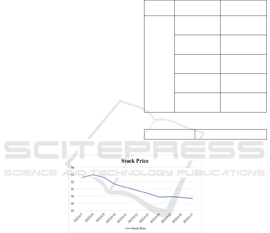
Figure 1: The historical stock price if Pfizer Inc.
This icon shows and indicates that Pfizer's stock
traded continuously during the trading day from June
7th to June 17th, and the stock traded at relatively
random prices.
3 METHODS
After selecting the above data, use the data to
construct three different option pricing models.
According to the different theoretical basis of the
models, the three models are divided into historical
data model, BS model, and BT model. The
construction ideas of the three models are roughly
similar, the difference is that the volatility is slightly
different. The historical data model uses historical
volatility, while the BS and BT models use implied
volatility.
The Black-Scholes model, also known as the
Black-Scholes-Merton (BSM) model, is one of the
most important concepts in modern financial theory.
This formula is based on consideration of the
theoretical value of derivatives of investment
instruments, other risk factors that affect value, such
ICEMME 2022 - The International Conference on Economic Management and Model Engineering
382

as time, are also considered (Hayes, 2022). Since its
birth in 1973, it has been an important application
tool in the history of options contract pricing. The
binomial option pricing model, another important
method for option valuation, was developed in 1979.
The core of this model is the usage iteration process,
which allows arbitrary nodes or points in time within
the time span between the valuation date and the
option expiration date (Chen, 2019). In this study,
three different option pricing models are used to
complete the hedging of option A to minimize the
impact of errors on the final data.
After the option pricing model is established, the
model needs to be calibrated with data, and all three
models use 𝝈 calibration. In the calibration model
stage, the ideas of the three model calibrations are
relatively unified, but they tend to be diversified in
performance. The idea is to bring the variable 𝝈 into
one or more formulas that can reflect the size of the
error value and bring it in according to the collected
data to form a formula based on the data and the
value of 𝝈. The result of the reaction is that under
different data, the error The size of the value. After
that, set 𝝈 as the independent variable, set the
formula representing the error value and its result as
the dependent variable, perform the calibration
operation, and obtain the 𝝈 when the minimum error
value is obtained, which is the final purpose of this
step. Detailed model specifications are shown below.
In Historical Data Model, S represents the stock
price, and k represents the date, which starts from
June 6 to June 17. Then k+1 represents the second
day based of the k. First, use equation (1) to get the
logarithm values of stock prices on each date. Then
use equation (2) to calculate the difference of
logarithm values between every two days. All the
results of equation (2) are used to take the variance
value of equation (3). Because the trading of stocks
and options only occurs on trading days, assuming
that there are 251 trading days in a year, bring it into
equation (4) to get the final 𝝈 value.
A=log𝑆
(1)
R=log(𝑆
)−log𝑆
(2)
𝑉𝑎𝑟=𝑣𝑎𝑟(log (𝑆
)−log𝑆
)
(3)
𝜎=
√
𝑉𝑎𝑟 251
(4)
In BS Model, σ represents implied volatility, t
represents time to maturity, S(t) represents the stock
price, K represents the strike price of the option, and
r represents the interest rate, which is assumed to be
2.8% in this model (The Fed - Selected Interest Rates
(Daily), 2020). First use equation (5) and equation
(6) to calculate value of 𝑑
and 𝑑
which are the
required elements for further calculation. Equation
(7) and (8) calculate the call and put price of the
option, and the 𝑁
(
𝑑
)
represents the normal
distribution of 𝑑
, 𝑁
(
𝑑
)
represents the normal
distribution of 𝑑
. After getting the values of the call
and put options, put them into equation (9) to
calculate the SSE (Residual sum of squares) error. C
represents the call option prices, which calculate
from equation (7), P represents the put option prices,
which calculate from equation (8), and 𝑃
represents
the corresponding market values. At last, when the
SSE value is the smallest, the desired 𝜎 value can be
obtained.
𝑑
=
1
σ
√
(𝑡)
ln
𝑆
(
𝑡
)
𝐾
+𝑟+
σ
2
𝑡
(5)
𝑑
=
1
σ
√
(t)
ln
𝑆
(
𝑡
)
𝐾
+𝑟−
σ
2
𝑡
=𝑑
−σ
√
t
(6)
𝐶𝑡,𝑆
(
𝑡
)
=𝑆
(
𝑡
)
𝑁
(
𝑑
)
−𝐾𝑒
𝑁
(
𝑑
)
(7)
𝑃𝑡,𝑆
(
𝑡
)
=𝐾𝑒
𝑁
(
−𝑑
)
−𝑆
(
𝑡
)
𝑁(−𝑑
)
(8)
𝑆𝑆𝐸=
(𝑃
−𝑃
)
𝑃
+
(𝑃
−𝑃
)
𝑃
(9)
In the BT Model, u represents the up coefficient
in binomial tree, d represents the down coefficient, t
represents time to maturity, p represents option
prices, and r represents the interest rate, which is
assumed to be 2.8% in this model. Calculate the up
and down coefficients of each level of the binomial
tree according to equations (10) and (11). Then bring
each coefficient into equation (12) to get the prices of
the option. Using equation (13), the calculated option
price and the corresponding stock price are brought
in to calculate the SSE error, when the SSE value is
the smallest, the desired σ value can be obtained
(Muroi, 2022).
𝑢=𝑒
√
(10)
𝑑=
1
𝑢
(11)
𝑝=
𝑒
−𝑑
𝑢−𝑑
(12)
𝑆𝑆𝐸=
(𝑃
−𝑃
)
𝑃
+
(𝑃
−𝑃
)
𝑃
(13)
After the above calculation process, the obtained
𝝈 value can be the variable value used after the
model has been calibrated. After the model has been
calibrated, it can be combined with Option A for
hedging. All three models use the delta hedging
Option Pricing and Risk Hedging in Current Financial Market: A Case for Pfizer
383

method. In this step, the hedging process of the
historical data model and the BS model is the same,
and the BT model is slightly different. For BS model,
p(t) represents the portfolio value, and using equation
(14) to get each p(t), then using equation (15) to
finish the hedging process. The BT model will
additionally use equation (16) in the hedging phase,
where S represents the option price. Collect the
results of the three model hedges, compare them, and
draw a conclusion.
𝑝
(
𝑡
)
=𝑝
(
𝑡−1
)
+𝑁(𝑑
)(𝑆
(
𝑡
)
−𝑆
(
𝑡−1
)
)
(14)
𝐿𝑜𝑠𝑠 𝑤𝑖𝑡ℎℎ𝑒𝑑𝑔𝑖𝑛𝑔(𝑡)
=𝑆
(
𝑡
)
−𝐾−𝑝(𝑡)
(15)
𝐻𝑒𝑑𝑔𝑒 𝑟𝑎𝑡𝑖𝑜=
𝐷
−𝐷
𝑆
−𝑆
(16)
4 RESULTS
According to the numerical results, the three models
have played a practical role in the manifestation of
the hedging effect, and the historical data model has
the best final effect in the presentation of the results.
Table 3: The gain/loss of holding one unit of the option on Pfizer Inc.’s stock with hedging by historical data model.
Days T-t T_A Stock A(put) Delta_A(put) Sell/Buy stock Cash
2022/6/6 1 39 0.1553785 53.19 1.338987 -0.285192551 0.285192551 16.508378
2022/6/7 2 38 0.1513944 53.28 1.284773 -0.279170686 -0.006021865 16.189375
2022/6/8 3 37 0.1474104 54.06 1.053795 -0.24084287 -0.038327816 14.119179
2022/6/9 4 36 0.1434263 53.27 1.229061 -0.276060889 0.035218019 15.996818
2022/6/10 5 35 0.1394422 51.31 1.83916 -0.381873758 0.105812868 21.427861
2022/6/13 6 34 0.1354582 48.82 2.950776 -0.540372814 0.158499056 29.168176
2022/6/14 7 33 0.1314741 47.75 3.536934 -0.613388331 0.073015517 32.65792
2022/6/15 8 32 0.12749 47.88 3.427221 -0.607455173 -0.005933157 32.377484
2022/6/16 9 31 0.123506 47.69 3.5134 -0.623120722 0.015665548 33.128186
2022/6/17 10 30 0.1195219 47.38 3.679893 -0.647319738 0.024199016 34.278431
According to the table above, the result of
hedging using the historical data model shows that
the final loss is $0.071472 per unit.
Table 4: The gain/loss of holding one unit of the option on Pfizer Inc.’s stock with hedging by BS model.
Days T-t T_A Stock A(put) Delta_A(put) Sell/Buy stock Cash
2022/6/6 1 39 0.1553785 53.19 1.233434 -0.278295356 0.278295356 16.035964
2022/6/7 2 38 0.1513944 53.28 1.181519 -0.272043762 -0.006251594 15.704668
2022/6/8 3 37 0.1474104 54.06 0.958312 -0.232535959 -0.039507803 13.570628
2022/6/9 4 36 0.1434263 53.27 1.129156 -0.268778694 0.036242735 15.502792
2022/6/10 5 35 0.1394422 51.31 1.730362 -0.378709777 0.109931083 21.145086
2022/6/13 6 34 0.1354582 48.82 2.844506 -0.544474042 0.165764266 29.240056
2022/6/14 7 33 0.1314741 47.75 3.438411 -0.620624141 0.076150098 32.879485
2022/6/15 8 32 0.12749 47.88 3.329489 -0.614415597 -0.006208543 32.585888
2022/6/16 9 31 0.123506 47.69 3.418796 -0.630684062 0.016268465 33.365367
2022/6/17 10 30 0.1195219 47.38 3.589578 -0.655785007 0.025100944 34.558372
According to the table above, the result of
hedging using the BS model shows that the final loss
is $0.102301 per unit.
ICEMME 2022 - The International Conference on Economic Management and Model Engineering
384

Table 5: The gain/loss of holding one unit of the option on Pfizer Inc.’s stock with hedging by BT model.
Days T-t T_A Stock A(put) Delta_A(put) Sell/Buy stock Cash
2022/6/6 1 39 0.1553785 53.19 0.733978 -0.232385794 0.232385794 13.094578
2022/6/7 2 38 0.1513944 53.28 0.694675 -0.22488392 -0.007501873 12.696339
2022/6/8 3 37 0.1474104 54.06 0.519476 -0.1794846 -0.04539932 10.243468
2022/6/9 4 36 0.1434263 53.27 0.659125 -0.220793512 0.041308912 12.445137
2022/6/10 5 35 0.1394422 51.31 1.19646 -0.355724826 0.134931314 19.369851
2022/6/13 6 34 0.1354582 48.82 2.320051 -0.570073709 0.214348883 29.836524
2022/6/14 7 33 0.1314741 47.75 2.960814 -0.66647809 0.096404381 34.443162
2022/6/15 8 32 0.12749 47.88 2.854744 -0.658574284 -0.007903806 34.06857
2022/6/16 9 31 0.123506 47.69 2.961679 -0.678597143 0.020022859 35.027261
2022/6/17 10 30 0.1195219 47.38 3.157355 -0.709127711 0.030530568 36.477707
According to the table above, the result of
hedging using the BT model shows that the final loss
is $0.278274 per unit.
5 DISCUSSION
As shown in the results section, the results of the
hedging strategy based on the historical data option
pricing model are the best, the results of the hedging
strategy based on the BS model are second only to
the former, and the results of the hedging strategy
based on the BT model are not satisfactory. The
methods of historical data and BS models in the
hedging stage are delta hedging, so the factor that
affects the hedging result is the definition of delta
value. In the evaluation method of delta, the
historical data model is obviously more accurate. The
values of the parameters of this model come from the
actual stock price and option data. The BS model is
subject to its formula principle, and the calculation
steps of many parameters are more responsible, and
the occurrence of errors can also be attributed to this.
When the BT model is established in the option
pricing model, the value of 𝝈 after calibration is
different from the value of the historical data model
and the BS model. At the same time, the hedging
process of the BT model is slightly different from the
above two models in steps, and the calculation steps
are slightly more. As the calculation steps increase,
the possibility of the existence of errors also
increases. The comprehensive analysis of the BT
model is unsatisfactory in the final hedging results
because of the large error of the 𝝈 value and the
added hedging step also increases the error.
6 CONCLUSION
This paper studies the use of different methods to
establish option pricing models for a single
company's stock, and conducts hedging, and analyzes
and discusses the different performances of different
pricing models in hedging. This paper selects the
options of Pfizer Inc. stock and uses historical data,
BS model, and BT model to establish option pricing
models. Use the Historical Volatility method to
calibrate the historical data model and use the
Implied Volatility method to calibrate the BS model
and BT model. After calibration, the historical data
model, the BS model, and the BT model use delta
hedging as the hedging method to complete the
hedging process. When comparing the results, the
hedging results of the historical data model
performed the best, with the smallest amount of loss
per unit. This study emphasizes that when hedging
stock options of the same company, hedging
strategies based on different option pricing models
perform differently, which is beneficial for investors
to flexibly use different hedging strategies and option
pricing models for portfolio investment.
REFERENCES
A. Hayes. What Is the Black-Scholes Model?
Investopedia, 2022.
https://www.investopedia.com/terms/b/blackscholes.as
p#:~:text=The%20Black%2DScholes%20model%2C
%20aka
E. Ekström, J. Tysk, J. The Black–Scholes equation in
stochastic volatility models. Journal of Mathematical
Analysis and Applications, 2010, 368(2), 498–507.
Option Pricing and Risk Hedging in Current Financial Market: A Case for Pfizer
385

G. Sarwar. The interrelation of price volatility and trading
volume of currency options. Journal of Futures
Markets, 2003, 23(7), 681–700.
https://doi.org/10.1002/fut.10078
G. Bakshi, N. Kapadia. Delta-Hedged Gains and the
Negative Market Volatility Risk Premium. The
Review of Financial Studies, 2003, 16(2), 527–566.
https://doi.org/10.1093/rfs/hhg002
J. Cao, B. Han. Cross section of option returns and
idiosyncratic stock volatility. Journal of Financial
Economics, 2013, 108(1), 231–249.
https://doi.org/10.1016/j.jfineco.2012.11.010
J. Chen. How the Binomial Option Pricing Model Works.
Investopedia, 2019.
https://www.investopedia.com/terms/b/binomialoption
pricing.asp
L. Xu, S. J. Deng, V.M. Thomas. Carbon emission permit
price volatility reduction through financial options.
Energy Economics, 2016, 53, 248–260.
https://doi.org/10.1016/j.eneco.2014.06.001
The Fed - Selected Interest Rates (Daily) - H.15 - May 22,
2020. URL: www.federalreserve.gov.
Y. S. Tian. A flexible binomial option pricing model.
Journal of Futures Markets, 1999, 19(7), 817–843.
https://doi.org/3.0.co;2-d">10.1002/(sici)1096-
9934(199910)19:7<817::aid-fut5>3.0.co;2-d
Y. Muroi, S. Suda. Binomial tree method for option
pricing: Discrete cosine transform approach.
Mathematics and Computers in Simulation, 2022, 198:
312-331.
ICEMME 2022 - The International Conference on Economic Management and Model Engineering
386
