
A Comparative Study of Traditional Linear Models and Nonlinear
Neural Network Model on Asset Pricing
Wen Wang
School of Finance, Southwestern University of Finance and Economics, Chengdu, 611130, China
Keywords: Asset Pricing, CAPM Model, Fama-French Three-Factor Model, RESET Test, Neural Network.
Abstract: Models in traditional asset pricing theories, such as CAPM and the Fama-French three-factor model, explain
the linear relationship between market returns, company size, company type, and return on assets. But in a
more complex financial market, the linear relationship contained in the above model may not hold. Therefore,
the main focus of this paper is to analyze the nonlinearity between stock excess return and its influencing
factors. The existence of nonlinearity is confirmed via the RESET test proposed by Ramsey. Then, the
nonlinear neural network model is used to further study the nonlinear relationship. Based on the data of the
A-share market, it is verified that there is a nonlinear relationship between stock excess returns and their
influencing factors, and the nonlinear neural network model shows better prediction performance than
traditional linear models.
1 INTRODUCTION
Modern asset pricing theory mainly focuses on the
difference between expected returns of different
assets and the dynamics of the market risk premium.
Among the large number of theoretical models in this
field, the capital asset pricing model (CAPM)
undoubtedly occupies an important position. It is the
cornerstone of modern financial economics and the
pillar of financial market price theory. The model was
developed from the theory of modern portfolio
selection (Sharpe, 1964; Lintner, 1969; Fischer,
1972).
With the continuous development in the research
fields of asset pricing theory, academic circles
gradually discovered that, in addition to a single risk
factor, the return on assets is also affected by the
company's market value and book-to-market ratio.
Combining these new findings, Fama and French
(Eugene, 1996) proposed a three-factor model that
combines the risk factor, size factor, and value factor
as an improvement of CAPM.
However, most of the traditional asset pricing
models, such as the CAPM model and the Fama-
French three-factor model, adopt a linear form and
usually have a problem with poor prediction of stock
returns. Therefore, the academic community has
gradually begun to explore the nonlinear relationship
in asset pricing models. According to empirical
research, there are complex internal structures in
asset price time series such as non-normal
distribution with fat tails, volatility clustering
phenomenon, and seasonal effects (Edgar, 1996; Xu,
2001; Michael, 1976). Faced with these nonlinear
characteristics, it is natural that reducing strict
assumptions in traditional models and building
nonlinear models becomes a new research direction
in the field of asset pricing (Xing, 2019; James,
2002).
This paper conducts an empirical analysis of the
traditional CAPM model, the Fama-French three-
factor model, and the neural network model based on
the A-share market data. Since it is confirmed that the
Fama-French three-factor model is more suitable for
the Chinese market than the Fama-French five-factor
model (Zhao, 2016), the Fama-French five-factor
model is not selected in this paper.
The Ramsey RESET method (James, 1969; Ruey,
2005) is used in the process to test whether there is a
nonlinear relationship between stock excess returns
and relevant factors under the single-factor
assumption and three-factor assumption,
respectively. Subsequently, the predicted stock return
of each model is compared via out-of-sample R2 and
mean absolute error (MAE).
In this paper, the nonlinear neural network model
is introduced to price assets in order to analyze the
Wang, W.
A Comparative Study of Traditional Linear Models and Nonlinear Neural Network Model on Asset Pricing.
DOI: 10.5220/0012036400003620
In Proceedings of the 4th International Conference on Economic Management and Model Engineering (ICEMME 2022), pages 535-541
ISBN: 978-989-758-636-1
Copyright
c
2023 by SCITEPRESS – Science and Technology Publications, Lda. Under CC license (CC BY-NC-ND 4.0)
535
nonlinear relationship between traditional pricing
factors and stock returns in the Chinese market. As a
result, the nonlinear problem existing in the
traditional linear asset pricing model is verified, and
the effectiveness of the neural network model applied
to the field of asset pricing is proven. The conclusions
obtained in this paper help to provide some guidance
for the improvement of the asset pricing model for the
Chinese market in the future.
2 MODELS
This section will introduce the pricing model used in
this paper. Pricing models are divided into two
categories: linear pricing models and nonlinear
pricing models.
2.1 Traditional Linear Models
Traditional asset pricing models generally take a
linear form. In this paper, the most classic CAPM and
the Fama-French three-factor models are selected for
empirical research.
CAPM. The single-factor CAPM formula
(including the market risk premium factor) is shown
below:
𝑅
−𝑅
=𝛼
+𝛽
𝑅
−𝑅
+𝜀
Among the equation above, R
represents the
rate of return of stock i at time t; R
is the risk-free
interest rate at time t; α
and β
are parameters to be
estimated; R
is the rate of return of the market
index at time t; ε
is the regression residual.
Fama-French three-factor model. Compared
with CAPM, the Fama-French three-factor model
includes two additional factors: stock market value
and book-to-market value. The formula of the model
(including market risk premium factor, size premium
factor and value premium factor) is shown below:
𝑅
−𝑅
=𝛼
+𝛽
𝑅
−𝑅
+𝛽
𝑆𝑀𝐵
+𝛽
𝐻𝑀𝐿
+𝜀
In the equation above, R
is the rate of return of
stock i at time t; R
is the risk-free interest rate at
time t; α
, β
, β
and β
are parameters to
be estimated; R
is the rate of return of the market
index at time t; SMB
represents the size premium at
time t, which is the difference between the return of a
portfolio of stocks with small market value and a
portfolio of stocks with large market value; HML
represents the value premium at time t, which is the
difference between the return of a portfolio of value
stocks and a portfolio of growth stocks at time t; ε
represents regression residuals at time t.
2.2 Nonlinear Neural Network Model
In order to further explore the nonlinearity between
stock returns and their influencing factors, the
nonlinear neural network model is introduced in this
paper.
Principle of the model. A neural network is one
of the most powerful nonlinear models in all kinds of
machine learning methods. The principle of the model
is to imitate the structure and function of a biological
neural network. As for the traditional feedforward
neural network, it mainly consists of an input layer for
raw data input, several hidden layers for processing
the input data, and an output layer that outputs the
final prediction results. Similar to the axons of a
biological brain, different layers in a neural network
model represent a group of neurons, and each layer is
connected by "synapses" that transmit signals between
neurons in different layers.
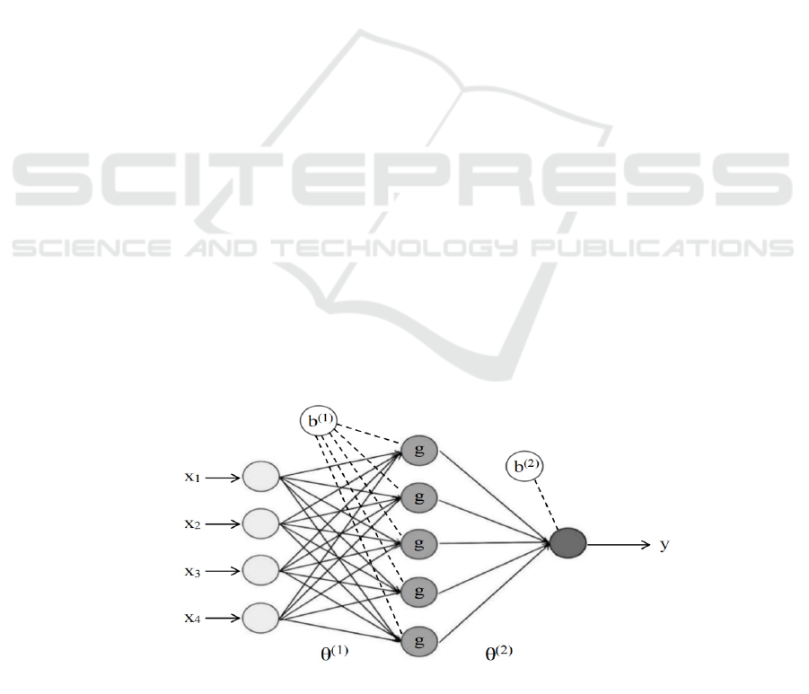
Figure 1: A single hidden layer neural network structure.
In
p
ut la
y
e
r
Hidden la
y
e
r
Out
p
ut la
y
e
r
ICEMME 2022 - The International Conference on Economic Management and Model Engineering
536

Figure 1 shows a single-hidden-layer neural
network structure. In this neural network structure,
x
, x
, x
and x
are the input data;θ
()
and θ
()
are the weight matrices mapped from the first layer to
the second layer and from the second layer to the third
layer, respectively; b
()
and b
()
are bias between
the first layer and the second layer, and between the
second layer and the third layer, respectively; g is the
nonlinear activation function; y is the final output
value. The overall structure of the model can be
expressed as equations below:
x
()
=g(𝜃
,
(
)
b
()
+𝜃
,
(
)
𝑥
)
𝑦=𝜃
(
)
𝑏
(
)
+𝜃
(
)
x
()
The form of the model. First, relevant data used
in asset pricing is expressed in vector form:
X
=
[
𝑥
⋯𝑥
]
𝑌
=[𝑦
…𝑦
]
In the equations above, X
is a dataset containing
m factors that impacts stock prices at time t; x
represents the ith factor at time t; Y
is the stock
excess return of n stocks at time t; y
represents the
excess return of stock i at time t.
Introducing the neural network into asset pricing,
a nonlinear model can be obtained as follows:
𝑌
=𝑓(X
;𝜃)
In this model, f is the nonlinear function that
maps the stock factor dataset X
to the excess return
Y
, and θ is the parameter set to be estimated.
3 EMPIRICAL ANALYSIS
The monthly data of 163 stocks selected from the A-
share market from January 2000 to May 2022 is used
in the paper to carry out the empirical experiment. All
stock data is obtained from the CSMAR database.
Stocks carrying “ST” (special treatment) or “*ST”
tags (which have suffered losses for two consecutive
years or more) are excluded. The market index used
here is the CSI 300 index, which includes the 300 A-
share stocks traded on the Shanghai and Shenzhen
stock exchanges, and the risk-free interest rate is the
one-year short-term treasury bond rate. The stock
data from January 2000 to December 2020 is used as
the training set of the pricing model, and the stock
data from January 2021 to May 2022 is used as the
test set.
3.1 Performance Evaluation
In order to compare the predictive ability of different
models, this paper selects two quantitative indicators:
R
2
and mean absolute error (MAE).
Out-of-sample R
2
. The predictive ability of each
model is evaluated by the out-of-sample R
2
:
R
=1−
∑
𝑟
,
−𝑟̂
,
(,)
∑
𝑟
,
(
,
)
In the formula above, r
,
represents the actual
excess rate of return of stock i at time t+1, and r
,
represents the excess rate of return of stock i at time
t+1 predicted by pricing models. Considering that
there is too much noise in the historical average excess
return of a single stock, it is better to directly use 0 as
the benchmark (Gu, 2020). Therefore, the
denominator of the out-of-sample R
2
defined here is
without demeaning, which means the historical mean
is replaced by 0.
Mean absolute error. In addition to R
2
, the
predictive ability of each model is also evaluated by
mean absolute error (MAE):
𝑀𝐴𝐸 =
1
𝑛
𝑟
,
−𝑟̂
,
In the formula above, r
,
represents the actual
excess rate of return of stock i at time t+1, and r
,
represents the excess rate of return of stock i at time
t+1 predicted by pricing models.
3.2 Nonlinearity Test
In this paper, regression specification error test
(RESET) is selected to detect the possible nonlinear
relationship in the model.
Testing method. The RESET test is a commonly
used test method in econometrics. It is a specification
test for linear least-squares regression analysis
proposed by Ramsey (1969). The basic idea of the
RESET test is that if there is no nonlinearity, the
coefficient of the multinomial term of the regression
model should be 0. In other words, the null hypothesis
of the RESET test is that the coefficient of the higher-
order term is equal to 0. This can be tested by the F
test.
Test result. The monthly excess returns of the 163
stocks selected in this paper are tested by RESET
under the assumption of a single factor (i.e. market
risk premium factor) and three factors (i.e. market risk
premium factor, size premium factor, and value
premium factor) respectively. The P values obtained
by the F test are shown in Table 1 and Figure 2.
A Comparative Study of Traditional Linear Models and Nonlinear Neural Network Model on Asset Pricing
537
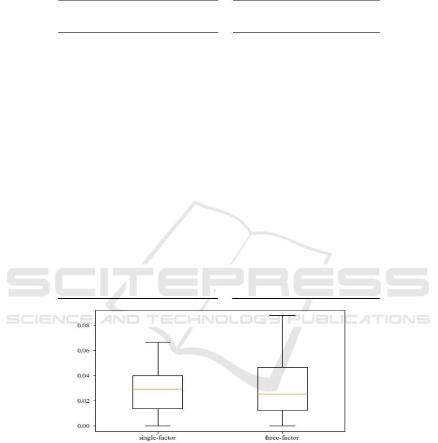
Table 1: Partial results of P value obtained by F test.
Stock
code
P value for
single-factor
P value for
three-factor
Stock
code
P value for
single-factor
P value for
three-factor
000012
0.0406 0.0170
000551
0.0118 0.0441
000021
0.0418 0.0368
000559
0.0664 0.0201
000026
0.0350 0.0681
000570
0.0062 0.0249
000039
0.0370 0.0292
000573
0.0434 0.0366
000055
0.0359 0.0493
000581
0.0140 0.0173
000060
0.0259 0.0110
000589
0.0350 0.0014
000078
0.0289 0.0466
000597
0.0072 0.0681
000089
0.0372 0.0135
000598
0.0197 0.0508
000402
0.0178 0.0333
000599
0.0377 0.0475
000404
0.0312 0.0242
000632
0.0639 0.1399
000417
0.0481 0.0342
000637
0.0129 0.0246
000419
0.0491 0.0161
000661
0.0159 0.0231
000422
0.0185 0.0023
000667
0.0090 0.0220
000425
0.0241 0.0148
000680
0.0378 0.0485
000507
0.0244 0.0242
000685
0.0274 0.0278
000521
0.0484 0.1164
000701
0.0083 0.0125
000528
0.0112 0.0483
000702
0.0080 0.0118
000543
0.0043 0.0171
000729
0.0178 0.0352
000548
0.0142 0.0034
000733
0.0242 0.0296
Figure 2: p value of the RESET test.
As shown in Table 1 and Figure 2, among the 163
selected stocks, P values of most stocks' excess
returns are less than 0.05. 92.64% of the stocks have
a P value less than 0.05 under the single factor
assumption, and 84.66% of the stocks have a P value
less than 0.05 under the three-factor hypothesis.
Hence, there are sufficient reasons to reject the null
hypothesis, that is, there are nonlinear terms in the
model under the single-factor and three-factor
assumptions. Consequently, it is reasonable to use
nonlinear neural network models to predict stock
excess returns.
3.3 Model Training
The stock data from January 2000 to December 2020
is used as the training set to estimate the parameters
of three different models, and the stock data from
January 2021 to December 2022 is used as the test set
to compare the performance of models via out-of-
ICEMME 2022 - The International Conference on Economic Management and Model Engineering
538

sample R
2
OOS
and MAE.
Linear Regression for Traditional Models. The
linear regression is performed on the training set data
to calculate the parameters of the CAPM and Fama-
French three-factor models. Part of results of each
model are shown in table 2 and table 3 respectively.
As can be seen from table 2 and table 3, the
regression coefficients of the market risk premium
factor are generally around 1, while the coefficients
of the size premium factor and the value premium
factor are basically distributed between 1 and -1.
Table 2: Partial CAPM Model Regression Coefficients.
Stock code β Stock code β
000012
1.3623
000551
1.0514
000021
1.0567
000559
1.1099
000026
1.0829
000570
1.1503
000039
1.0150
000573
1.1043
000055
1.1454
000581
0.9272
000060
1.4895
000589
1.0393
000078
1.2271
000597
1.0332
000089
0.9121
000598
1.0690
000402
0.9913
000599
1.1078
000404
1.0987
000632
0.9774
000417
0.9409
000637
0.9588
000419
1.0821
000661
1.0209
000422
1.1367
000667
1.1438
000425
1.0501
000680
1.3344
000507
1.1369
000685
1.3469
000521
1.1357
000701
1.1495
000528
1.2415
000702
0.9878
000543
1.2621
000729
0.6887
000548
1.2354
000733
1.1190
Table 3: Partial FF three-factor model regression coefficients.
Stock
code
βM βSMB βHML Stock
code
βM βSMB βHML
000012
1.2984 0.8745 0.2684
000551
0.9667 1.0525 0.1440
000021
0.9835 0.6161 -0.4609
000559
1.0265 1.0905 0.2469
000026
0.9729 1.0106 -0.5234
000570
1.0791 0.8716 0.0944
000039
1.0365 -0.1216 0.2529
000573
1.0465 0.9281 0.5163
000055
1.0565 1.0752 0.0905
000581
0.8934 0.3855 -0.0135
000060
1.4956 0.0598 0.2589
000589
0.9865 0.8760 0.5254
000078
1.1373 0.9139 -0.2511
000597
0.9531 1.1435 0.4302
000089
0.8898 0.2253 -0.0658
000598
1.0308 0.6422 0.3988
000402
1.0414 -0.4816 0.1966
000599
1.0207 1.1217 0.2238
000404
1.0260 1.0489 0.4129
000632
0.8818 1.0587 -0.0961
000417
0.8932 0.7500 0.3928
000637
0.8985 0.8616 0.3242
000419
1.0099 0.7348 -0.1998
000661
0.9102 1.1682 -0.2256
000422
1.1040 0.6689 0.5791
000667
1.1074 0.7903 0.7325
A Comparative Study of Traditional Linear Models and Nonlinear Neural Network Model on Asset Pricing
539

000425
1.0329 0.4887 0.5753
000680
1.3322 0.1623 0.2709
000507
1.0981 0.5070 0.1139
000685
1.3244 0.3403 0.1592
000521
1.0679 0.9031 0.2354
000701
1.0545 1.0158 -0.1671
000528
1.2709 -0.2598 0.1607
000702
0.9178 1.0581 0.4926
000543
1.2454 0.4936 0.5963
000729
0.6727 0.1638 -0.0433
000548
1.1806 0.7695 0.2683
000733
1.0211 0.6783 -0.9043
Linear Regression for Traditional Models.
Considering the limited amount of data, the neural
network models used here have only up to 4 hidden
layers. Four neural network structures (NN1, NN2,
NN3 and NN4) are selected respectively according to
the geometric pyramid rule [13]. NN1 has a single
hidden layer with 32 neurons; NN2 has two hidden
layers with 32 and 16 neurons, respectively; NN3 has
three hidden layers with 32, 16, and 8 neurons,
respectively; NN4 has four hidden layers with 32, 16,
8, and 4 neurons respectively. Under the single-factor
assumption, the input layer of each neural network
model receives market risk premium data; under the
three-factor assumption, the input layer receives
market risk premium, size premium and value
premium data.
3.4 Model Comparison
The R
2
OOS
and MAE of CAPM and the neural
network model under the single-factor assumption is
shown in Table 3. It can be seen that the performance
of neural network models with all four different
structures is better than CAPM. The R
2
OOS
and MAE
of the Fama-French three-factor model and the neural
network under the three-factor assumption are shown
in Table 4. The neural network model also shows
better performance than the linear three-factor model
does.
Table 4: R
2
OOS
and MAE under the single-factor assumption.
Model CAPM NN1 NN2 NN3 NN4
R
2
OOS
0.1271 0.1307 0.1308 0.1300 0.1300
MAE 0.0799 0.0795 0.0795 0.0796 0.0795
Table 5: R
2
OOS
and MAE under the three-factor assumption.
Model FF NN1 NN2 NN3 NN4
R
2
OOS
0.2261 0.2287 0.2274 0.2278 0.2302
MAE 0.0741 0.0740 0.0737 0.0737 0.0736
4 CONCLUSION
Through empirical method, according to A-share
market data, the Ramsey RESET method is used in
this paper first to confirm that there is a nonlinear
relationship between the stock excess return and its
influencing factors. Then, from the results of both R
2
and MAE, we can see that all four nonlinear neural
network models with different structures show better
performance than traditional linear asset pricing
models. Hence, it is further verified that the non-
linear form may be a better option when it comes to
predicting asset returns.
However, the improvement of the neural network
model over traditional linear models is not very
significant. In addition, it is difficult to give an
intuitive explanation of the specific nonlinear
relationship between expected returns and their
influencing factors via a neural network model
because it is like a “black box”. Consequently, other
nonlinear models are needed to further explore the
nonlinear relationship between stock excess return
and relevant factors.
REFERENCES
Edgar, E., Peters. (1996). Chaos and Order in the Capital
Markets: A New View of Cycles, Prices, and Market
Volatility.
ICEMME 2022 - The International Conference on Economic Management and Model Engineering
540

Eugene, F., Fama., Kenneth, R., French. (1996).
Multifactor Explanations of Asset Pricing Anomalies.
Journal of Finance, 51(1):55-84.
Fischer, Black. (1972). Capital Market Equilibrium with
Restricted Borrowing. The Journal of Business,
45(3):444-455.
James, Davidson., Timo, Teräsvirta. (2002). Long memory
and nonlinear time series. Journal of Econometrics,
110(2):105-112.
James, B., Ramsey. (1969). Tests for Specification Errors
in Classical Linear Least-Squares Regression Analysis.
Journal of the royal statistical society series b-
methodological, 31(2):350-371.
Lintner, J. . (1969). The valuation of risk assets and the
selection of risky investments in stock portfolios and
capital budgets *. Stochastic Optimization Models in
Finance, 51(2), 220-221.
Michael, S., Rozeff., William, R., Kinney. (1976). Capital
market seasonality: The case of stock returns. Journal
of Financial Economics, 3(4):379-402.
Ruey, S., Tsay. (2005). Analysis of Financial Time Series:
Tsay/Analysis of Financial Time Series.
Sharpe, W. F. . (1964). Capital asset prices: a theory of
market equilibrium under conditions of risk*. Journal
of Finance, 19(3), 425-442.
Shihao, Gu., Bryan, T., Kelly., Dacheng, Xiu. (2020).
Empirical Asset Pricing via Machine Learning. Review
of Financial Studies, 33(5):2223-2273.
Xu, L. . (2001). Empirical Research on the Stable
Properties of Stock Return in China Stock Market.
Journal of Financial Research(06), 36-43.
Xing, H. , & Liu, W. . (2019). Nonlinear asset pricing
model and the idiosyncratic volatility puzzle. Journal of
Systems Engineering.
Zhao, S. , Yan, H. , Kai, Z. , Finance, S. O. , & University,
N. . (2016). Does fama-french five factor model
outperform three factor model? evidence from china's
a-share market. Nankai Economic Studies.
A Comparative Study of Traditional Linear Models and Nonlinear Neural Network Model on Asset Pricing
541
